Global Optimization Approaches to Generate Dynamically Robust Electrophysiologic Models

Introduction

The electrical activity underlying the cardiac action potential emerges from a complicated process. It involves a large number of proteins including ionic channels and transporters that often have nonlinear dependencies on components such as the transmembrane potential and the concentration of ionic species. As an additional level of complexity, different components influence one another through feedback loops. Complex systems such as this often exhibit emergent properties that are not easily predicted from the characteristics of the individual parts. Consider, as an example, triggering of early afterdepolarizations in a cell caused by a block of the rapid delayed rectifier potassium current (I _Kr ). Whether this proarrhythmic event is triggered or not depends not only on the extent of I _Kr block in a particular cell, but also on the availability of compensating current (such as the slow delayed rectifier potassium current, I _Ks ), and on the exact activities of the inward currents that actually generate the afterdepolarization (i.e., the L-type calcium current [I _CaL ] and/or sodium-calcium exchange current [I _NCX ]), which in turn have additional dependencies on the dynamic intracellular calcium concentration.

Because of this complexity, mathematical models of cardiomyocyte electrophysiology are valuable tools for illumination of both normal and pathophysiologic electrical activity, as a model allows access to all variables at all time points during specific interventions. A large number of cardiac cell models have been developed over the last decades, generally incorporating an increasing level of detail and specificity. ^, Model applications have a wide span, including making predictions regarding anti- or proarrhythmic effects of pharmacologic agents, illuminating ionic mechanisms underlying arrhythmias, and studying consequences of genetic variations.

Limitations to Cardiac Ionic Model Development Process

Unfortunately, the reality of mathematical modeling does not always live up to the potential just described. Models have in many cases been applied successfully but often fail to accurately simulate complex dynamics. Two examples are (1) the rate dependence of the action potential is inaccurate for several human atrial and ventricular cell models, and (2) models may not exhibit expected arrhythmia-relevant dynamics such as early afterdepolarizations and repolarization alternans. ^, We believe that several limitations, inherent to the traditional model-development process, contribute to these deficiencies :

1.
Interlaboratory variations and data inconsistency. Models are typically constructed based on voltage-clamp data of individual currents. For several reasons, including specialization in biological interests and experimental techniques, these data usually come from multiple laboratories. Therefore the data have often been obtained under different experimental protocols (with varying conditions such as temperature and solution composition) and from animals or subjects with divergent characteristics (including sex, age, and breed of animals), which are all factors that affect cellular electrophysiology.
2.
Intercell variability. In addition to such externally imposed variations, individual cardiac myocytes exhibit intrinsic cell-to-cell variability in electrical activity. Even cells originating from the same region of a given heart form a heterogeneous population. ^, Both local cell-to-cell and interheart biological variability in electrophysiologic properties are typically disregarded when formulating mathematical cardiomyocyte models, which instead rely on population-averaged data to generate a “representative” model. However, the extent to which such a model actually represents a heterogeneous population is unknown; moreover, the fidelity of an average model in predicting the effects of perturbations to a particular cell (e.g., the response to a pharmacologic agent) is limited. ^,
3.
Manual parameter tuning. Average voltage-clamp data are combined with equations for the individual currents to build a composite model. This is a step that often requires adjustment of model parameters for the model to reproduce desired whole-cell behavior. This tuning is typically done manually by tweaking parameters (typically the conductances) in a cumbersome process until the model generates output that is deemed to reproduce the desired target behavior. However, an automated search heuristic, which can test many more parameter combinations in a directed manner, is much more likely to find the best fit to the data.
4.
Dynamically simple data. The data to which models traditionally have been tuned are typically relatively simple (such as a single action potential). However, a host of different parameter combinations may in fact result in simple outputs that appear equivalent, and dynamically simple data are therefore insufficient at uniquely identifying model parameters. ^, Consequently, a model tuned to simple data would not be expected to accurately predict the more complex dynamics associated with cardiac arrhythmias, as different channel compositions change many properties of electrical activity. This is a severe limitation, as one of the fundamental ambitions of cardiac modeling is to illuminate mechanisms underlying arrhythmias.

Using Complex Electrophysiologic Protocols and Optimization to Generate Models

Recently, two central strategies have been applied in efforts to overcome these inherent limitations to model development: use of automated, global search methods and use of rich target data. The two strategies work best when combined, in which case they generate a powerful parameter estimation methodology.

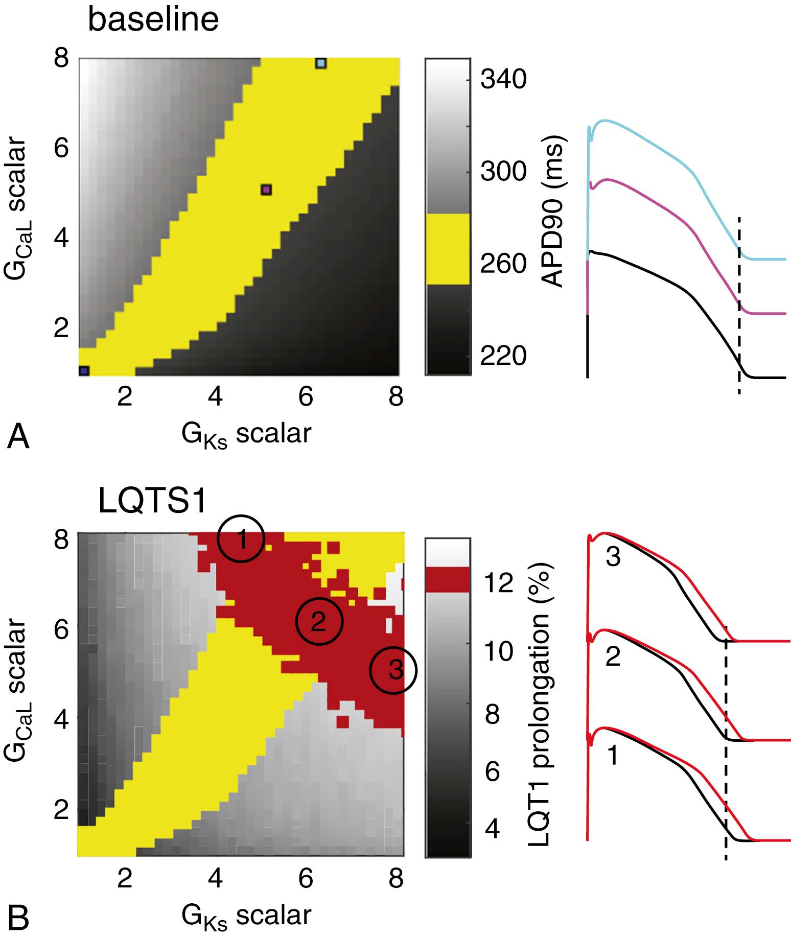
To see in more detail why more complex data are advantageous for model development, consider the following. The action potential is generated from the algebraic sum of many inward and outward currents. Its duration is largely controlled by the relatively small net outward current during the slow repolarization associated with phase 2 of the cardiac action potential. This net current can come about by a near-balance of a range of levels of the individual inward and outward currents, with different amounts of cancellation between opposite-going currents and compensation among similar currents. This idea is exemplified in Fig. 31.1A , which shows that combinations of I _CaL and I _Ks conductances may generate action potentials with nearly identical durations. However, the response to perturbations will not be equivalent among cells or models using different current combinations. For example, the response to decreased I _Ks conductance (to simulate long QT type 1 syndrome) would give rise to different amounts of action potential prolongation (see Fig. 31.1B ). Therefore use of this data as an additional target during model development effectively reduces the range of parameter combinations that produce acceptable outputs.

Fig. 31.1, Additional objective data constrains parameters.

Genetic Algorithm Optimization

For the purpose of estimating parameter values in models, solving an optimization problem means determining the set of parameters that minimizes the difference between model output and target data. As discussed in this section, the genetic algorithm is a search method that is highly suitable for finding such solutions.

The genetic algorithm is one of several optimization strategies inspired by evolutionary dynamics. The premise behind the genetic algorithm is that an initial pool of random parameter sets evolve toward a best parameter set by means of computational correlates of (1) survival of the fittest (i.e., selection of parameter sets resulting in model output closest to the target objective), (2) reproduction and generations (pairing of parent models to create new offspring models), (3) crossover (parameter exchange), and (4) mutation (parameter modification).

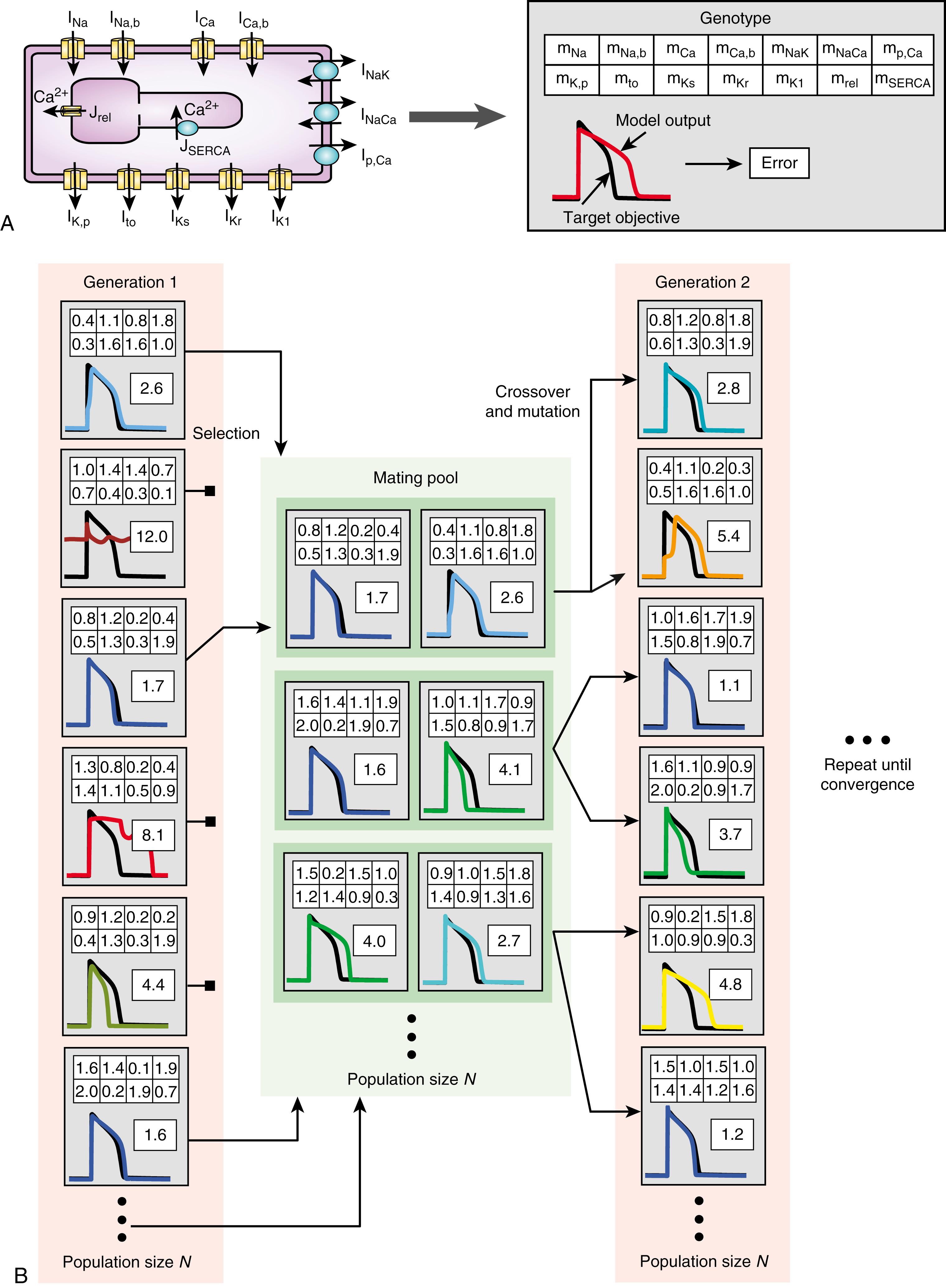
How these operations guide the evolution of parameter sets is shown in Fig. 31.2 , which is an application of a genetic algorithm to estimate parameters in a cardiac electrophysiology model. In this representation, the genes of the genetic algorithm are the parameters to be estimated; here they include maximal conductances or fluxes of the ionic channels and transporters (see Fig. 31.2A ). Different model instantiations, or individuals in the context of biological evolution, will have different combinations of these gene values. For each individual, an output can be obtained by simulating the model with its particular set of parameter values. This output can then be compared with the desired target objective, resulting in an error measure (see Fig. 31.2A ). Note that the progression of the genetic algorithm to minimize this error correlates with the notion of maximizing an opposite fitness measure in Darwinian evolution.

Fig. 31.2, Schematic of genetic algorithm principles.

The genetic algorithm starts out with a population of models with randomized parameter values (see Fig. 31.2B ). A selection process then eliminates individuals based on their error values, such that poorly matching solutions are discarded. The surviving models form a mating pool and are recombined to generate new offspring models in the process of crossover. One way to implement this process is by a so-called uniform crossover (illustrated in Fig. 31.2B ), in which parameters from two parents are swapped on a gene-by-gene basis with equal probability between two children. After crossover, the genes of the offspring may undergo mutation to generate new values (see Fig. 31.2B ).

The processes of selection, crossover, and mutation are repeated through generations of model pools, until a convergence or stop criterion is reached (e.g., that the reduction in error between consecutive generations is less than a set value or that the error of the best individual is below a certain threshold).

In addition to the randomization of the parameters of the individuals in the first generation, genetic algorithms rely on stochastic processes during the simulated evolution to maintain population diversity and prevent the search from converging on a suboptimal solution (i.e., a local, rather than the global, minimum of the error in the parameter search space). Elements of randomness can be incorporated into all the key operations of the algorithm. For example, for the selection process, we use a pairwise tournament selection; this method randomly pairs two individuals and chooses the one with the lower error to continue to the mating pool while discarding the other. How mating pool members are combined, how genes are interchanged when generating offspring, and how genes are mutated also readily succumbs to randomization.

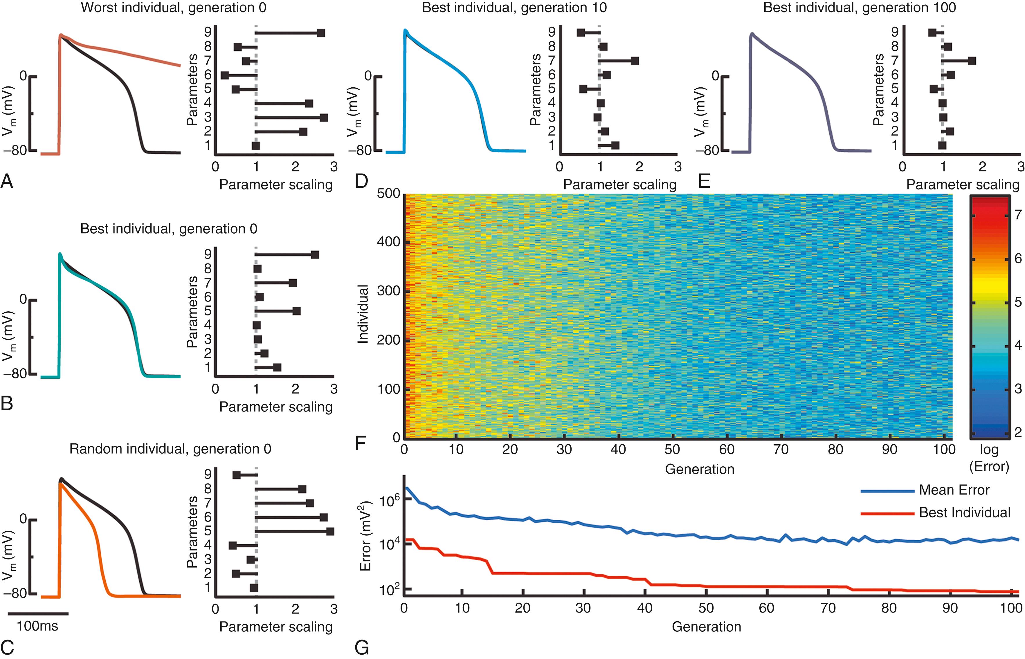
Example: Genetic Algorithm Optimization to Single Action Potential

A specific example of parameter estimation by a genetic algorithm in an ionic cardiomyocyte model is shown in Fig. 31.3 . In this case we illustrate the performance of the genetic algorithm by fitting the model to its own output, such that the optimization should return the known parameters. The particular model is the guinea pig ventricular myocyte model created by Faber and Rudy.

Fig. 31.3, Genetic algorithm optimization to single action potential objective.

In this setup, each generation consists of 500 individuals. As their parameters are randomized, most individuals generate output that is very different from the single action potential target (see Fig. 31.3A and C ). However, some model instantiations fit the target well by chance (see Fig. 31.3B ). As the optimization progresses, errors decrease as fits get closer to the target (see Fig. 31.3F–G ). For example, in the 10th generation, the model with the lowest error produces an action potential that is almost identical to the objective (see Fig. 31.3D ), and in the 100th generation, the best fit is essentially indistinguishable from the target (see Fig. 31.3E ).

Importantly, the closest reproduction of the target found by the genetic algorithm is not obtained through a complete recovery of the known parameters (i.e., a parameter scaling of 1 in Fig. 31.3 ). In particular, the conductance of the plateau potassium current (parameter 7) is overestimated, whereas I _Kr conductance and maximal SERCA flux (parameters 5 and 9) are underestimated. This exactly exemplifies the situation in Fig. 31.1 , where different combinations of parameter values can produce nearly identical action potentials. Although it is possible that continuing the progression of the genetic algorithm would eventually lead to more accurate recovery of these parameters, it is likely that using a single action potential as the target simply provides insufficient information to constrain the parameter better.

You're Reading a Preview

Become a Clinical Tree membership for Full access and enjoy Unlimited articles

Become membership

If you are a member. Log in here