Artificial Intelligence and Radiology

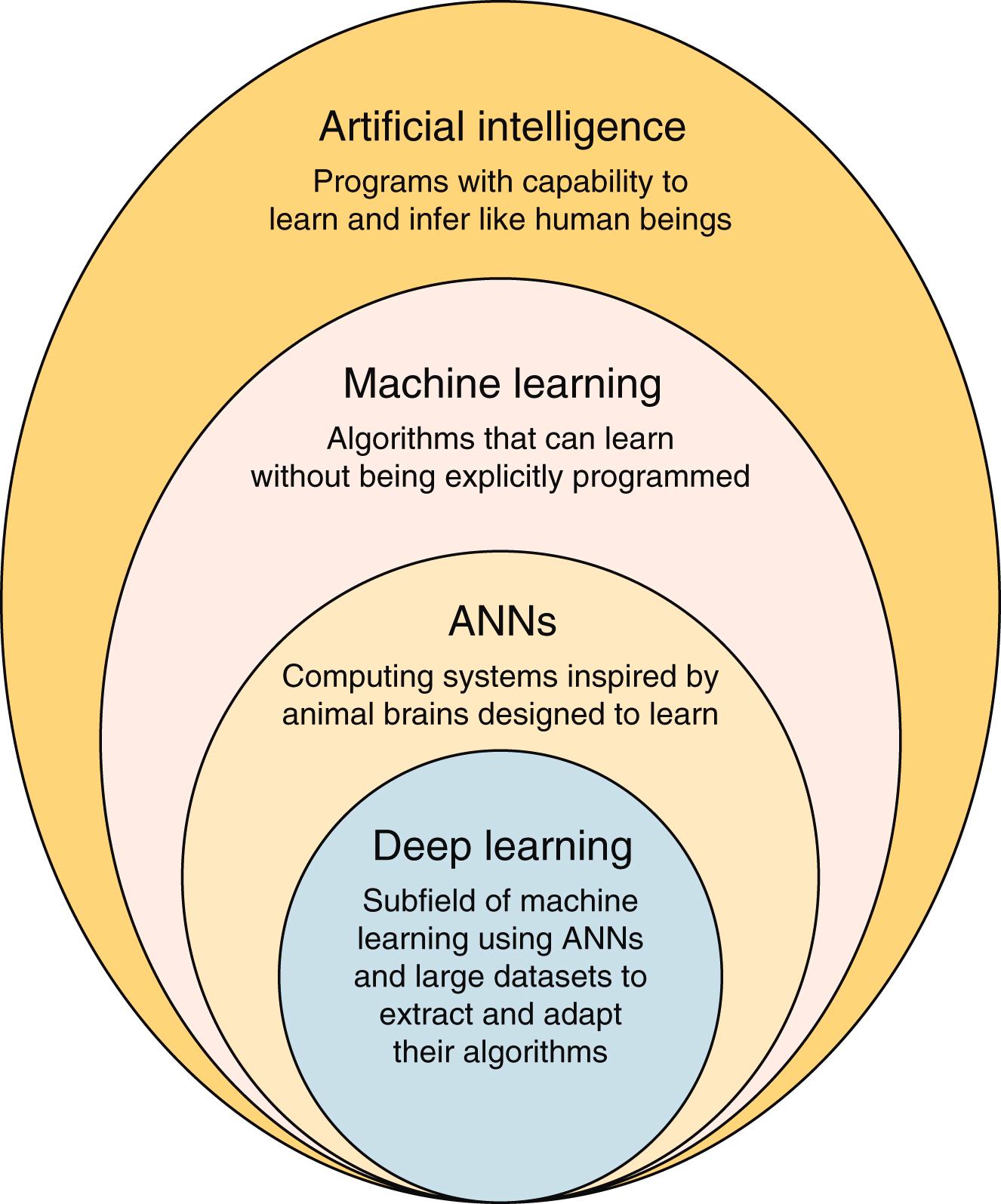
Artificial intelligence (AI) is the field of computer science that involves the simulation of intelligent behavior by computers. It is used to predict, automate, augment, and optimize tasks historically done by humans.

To provide an overall view of some of the key terms and their relationships to each other, see eFig. G.1 (each will be discussed in this chapter).

The lack of computer processing power along with difficulty accessing appropriate amounts of training data affected the early progress of AI.

Artificial intelligence requires a vast amount of computational power to process its data. AI could not be possible without a quantum leap in computer processing power.

At the time of the Dartmouth Conference in 1956, the most advanced computer was built by IBM. It occupied an entire room , stored its data on cassette tapes, and received its instructions using paper punch cards.

In 2020, the iPhone 12, which, by comparison, fits in the average person’s pocket , could perform 11 trillion operations per second, which is 55,000,000 times more than the IBM computer in 1956.

And in 2018, what was then the world’s fastest modern supercomputer could perform a computation in 1 second that would have taken the “old” IBM almost 32,000 years to compute.

A major part of that increase in computational speed came from the realization that the hardware known as graphics processing units (GPUs) could greatly accelerate processing speeds because of their ability to quickly manage large blocks of data simultaneously ( eBox G.1 ).

Artificial neural networks ( neural networks or ANNs ) are inspired by the neural networks in animal brains and based roughly on the way the human brain is believed to work.

As our own neurons receive electrical signals from other neurons, the electrical energy inside of their cell bodies increases until a certain threshold of activation is met, at which point the electrical signal travels down the axon and is delivered to another neuron. This process is repeated many times. Through each neuron’s dendrites , a single neuron in the brain connects to many thousands of other neurons.

In an ANN, collections of software neurons (called nodes or neurons ) are connected to each other and configured so that they can send messages to each other. The receiving (postsynaptic) node processes its signal(s) in the form of numbers or bits that computers can use and then, in turn, sends signals to downstream nodes connected to it. Every node is connected to every other node in the next layer and every connection has its own weight.

• Weights are the means by which ANNs learn. Through adjusting the weights, the ANN decides to what extent signals get passed along. This weight can change as learning proceeds, which in turn increases or decreases the strength of the signal that nodes transmit downstream.

A neural network may consist of thousands or even millions of simple processing nodes that are interconnected.

These systems learn (i.e., increasingly improve their ability) to do tasks by analyzing examples, mostly without task-specific programming.

• For example, a set of training data may have been hand-labeled in advance and consist of thousands of tagged images of boats, cars, and planes, but the network would find its own visual patterns in those images that reliably correlate with each of their tags in order to classify them into their appropriate categories.

In radiology, specialized ANNs might learn to identify images that contain lung nodules by analyzing example images that have been manually labeled as lung nodule and using the learned results to identify lung nodules in other, unknown images.

The neural network is asked to solve a problem time and again, each time strengthening the connections that lead to success and reducing those connections that lead to failure.

Most modern deep learning models are based on artificial neural networks.

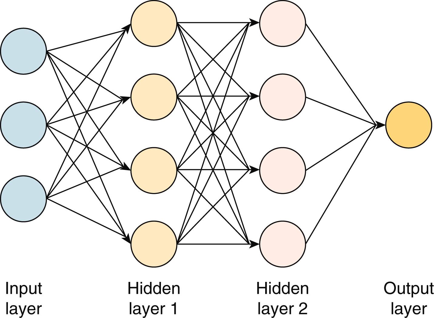
To perform these analyses, nodes are typically organized in groups, called layers ( eFig. G.2 ) .

The input layer may be an image, or parts of an image. Then, there are several hidden layers that have the function of extracting image features. Lastly, there is the output layer , which answers the question the network is designed to answer.

Each node receives an input, does a calculation, and outputs a value on to the next layer. The input of each node is made up of the output from all nodes in the previous layer. Traditionally, the hidden layers are fully connected —that is, every node in the first hidden layer is connected to every node in the second layer, which is, in turn, connected to every node in the third layer, and so on.

Part of the calculations each node makes involves determining the weights of its output, which have a direct influence on how input data is transformed and passed on from one node to the next. The process of determining the value of the weights, which will eventually provide the correct output, is the process called training.

To train a deep neural network correctly, example data (such as images) make up the input, and the corresponding correct output is the known correct answer for that image—the ground truth.

The training procedure is usually performed using three datasets that are independent of each other in that they should all contain different examples. They are: a training set, a validation set, and a test set . These datasets are used in three different steps of the training process ( eBox G.2 ).

The difference between the output of the model and the ground truth can be expressed as an error . For example, imagine our network is supposed to compute the probability that an image contains a lung nodule. An image containing a known lung nodule is fed into the system and the network produces a result that says 20% chance of lung nodule. We know that the best answer, in this case, should be 100% chance of lung nodule. We recognize this is an error of 80%, meaning there is more work to be done.

• This error calculation is done for each image in the training set and combined to obtain the total error of the network over the entire training set by summing up the errors for all images in the training set.

To minimize this total error, several methods are used, one of which is called backpropagation, which is achieved by adjusting all weights beginning at the output layer and working backward to the input layer. The system does this by finding which weights were responsible for the errors and changing those weights accordingly.

This training procedure should eventually produce a model that has a very small error when employed using the set on which it was trained (i.e., the training set ).

However, what might occur during this part of the training is that the network learns too much from the examples in the training set, unknowingly identifying patterns in not only the signal but the noise as well and assuming the noise was inherent in the underlying structure of the input. This results in an impressive performance on the training set but a weak performance when fed new data. This is called overfitting, and it means the network’s performance is not generalizable.

To help identify and adjust for overfitting, another independent dataset is used to assess the network’s performance. That dataset is called the validation set. Use of the validation set is done during the training process to see how well the model performs on data it has never seen. If the network performs well on the original training set but poorly on the validation set , there is overfitting, and adjustments will have to be made using either additional data or other processes.

The last step uses still another data set that has also not been seen by the network before, the testing set. The algorithm processes the images in the test set and its performance, e.g., its accuracy in finding a nodule, is calculated. This is an objective test of how the algorithm performs on data previously unseen by the network ( eBox G.3 ).

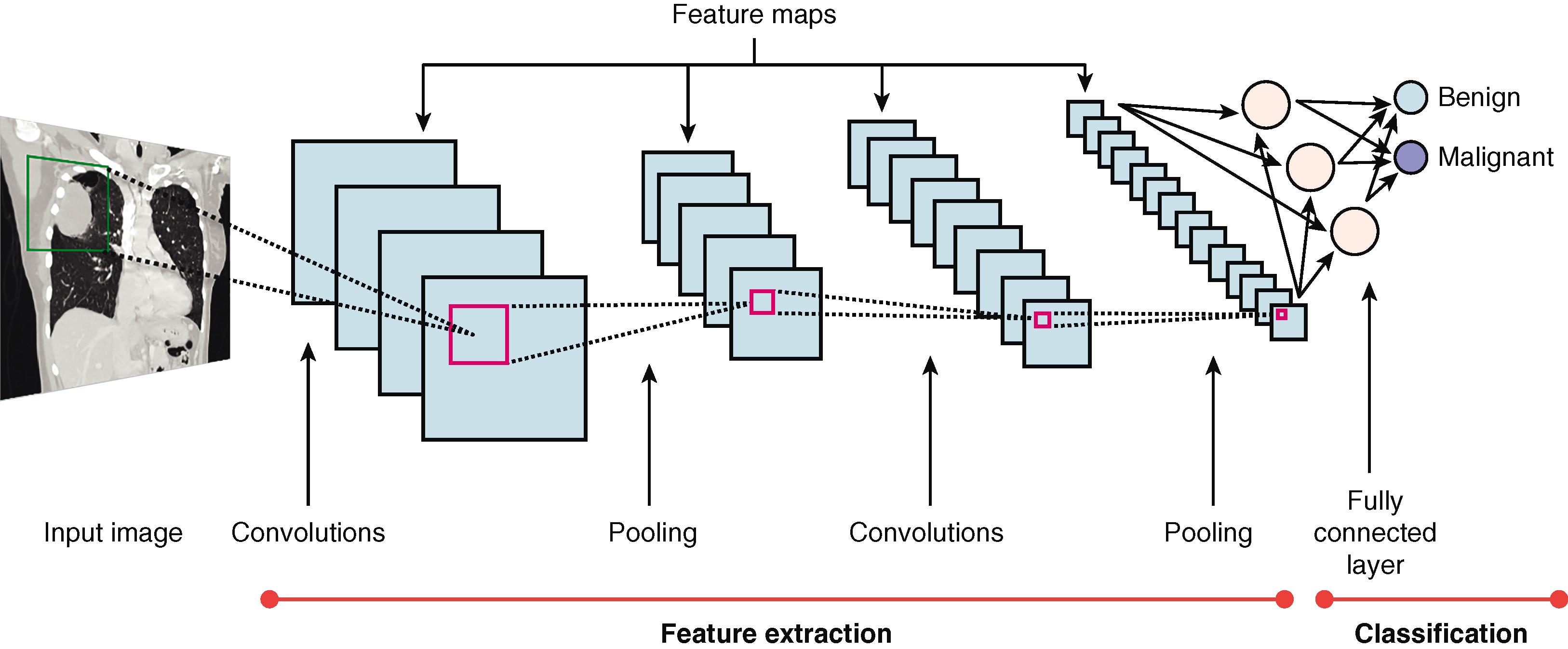
Convolutional neural networks (CNN or ConvNet) deserve a special mention because they are the most prevalent artificial neural network architecture in use for medical imaging processing. They were inspired by an animal’s visual pathways and they are efficient in object detection ( feature extraction ) and image classification.

CNNs make the explicit supposition that their inputs are images. This allows for the encoding of certain properties into the architecture of the system and alleviates certain preprocessing.

Convolutional neural networks apply multiple filters to an input image to create a pixel-by-pixel feature set that summarizes the presence and properties of detected objects from the input image. CNNs can look at groups of pixels in an area of an image and learn to find spatial patterns. They perform this extraction through a mathematical process known as convolution.

The filters are very small grids of values that systematically scan across the entire input image , pixel by pixel, and produce a filtered output that, at first, will be about the same size as the input image. The system repeatedly scans each output from a convolution layer, pooling the results into progressively smaller samples.

Pooling addresses the sensitivity CNNs have to learning the precise position of a feature in the feature map. Slight changes in the position of the input in subsequent examples could lead the system to produce multiple maps for the same feature, something that would not be helpful.

A pooling layer is a new layer added after the convolutional layer that decreases the size of the feature map, reducing the computation required by the network and making the model more robust to variations in changes to position of the features in the input image.

At the end of a convolutional neural network is at least one fully connected layer. Fully connected means that every output that is produced at the end of the last subsample is an input to each node in this fully connected layer.

It is here that the feature map outputs are sent for classification.

Classification takes the features from the output of the convolution layers and determines whether the output is a member of a class (e.g., a lung nodule or not a lung nodule ) or a probability that it is a member of a particular class (e.g., 80% chance this is a malignant lung nodule ) ( eFig. G.3 ).

CNNs are at the heart of nonmedical image classification as well, from tagging a face on Facebook to security and self-driving cars.