Physical Address
304 North Cardinal St.
Dorchester Center, MA 02124
This chapter includes an accompanying lecture presentation that has been prepared by the authors: ![]() .
.
This chapter includes an accompanying lecture presentation that has been prepared by the authors: ![]() .
.
Diagnostic and screening tests include measurements of validity and reliability. Validity examines sensitivity, specificity, positive predictive value (PPV), negative predictive value (NPV), and likelihood ratios (LRs); reliability refers to intrasubject variation, intraobserver variation, and intersubject variation, including percent agreement and kappa statistic (κ).
Appropriate study designs in establishing causation include case reports and case series, cross-sectional studies, cohort studies, case-control studies, literature reviews, and systematic reviews. Various types of confounding pertinent to these study designs are discussed.
Evaluating interventions/preventions typically requires randomized clinical trials and meta-analyses that lay the foundation for class I evidence.
A bayesian approach provides a 2 × 2 table that can be used with a majority of core epidemiologic concepts in neurosurgical research.
This chapter gives a broad overview of epidemiologic and biostatistical principles in neurosurgery. Although the appropriate breadth of these topics extends far beyond the scope of this chapter, our intention is to provide a framework for neurosurgeons who are not only evaluating the literature but also participating in clinical research that is published for the specialty. References are provided throughout the chapter, should the reader choose to pursue a greater amount of information with further details.
The two overarching themes of this chapter are epidemiology and biostatistics. Epidemiology has three sections, based on the type of study question: (1) diagnostic and screening tests; (2) establishing causation, in which study designs are outlined; and (3) evaluating interventions/preventions. The chapter ends with core concepts in biostatistics necessary to mathematically analyze any of the three aforementioned study questions. To assist readers in translating theory into practice, this chapter references a series of studies on cerebrospinal fluid (CSF) shunting, which serves as a relatable example for both adult and pediatric neurosurgery.
In epidemiology, measurements of a novel test must account for validity and precision. In Fig. 76.1 , validity refers to the accuracy of a test measure, whereas precision refers to the reliability of a test. Some common measures previously validated in neurosurgery have been discussed in the prior version of this chapter.

Validity measures the accuracy of the test. Perfect accuracy is defined as the “gold standard,” or the best single test for diagnosing a disease. A new test is usually compared against the gold standard, which is set a priori by the study investigators. Comparison between a new test and a gold standard can be calculated quantitatively with a bayesian table. For example, in patients with infected shunt occlusions, a gold standard was isolation of microorganisms in the blocked portion of the shunt apparatus, which would require surgical removal of the hardware. Because such an invasive procedure is not practical for every patient suspected to have an infected shunt occlusion, culturing of the CSF from the reservoir may serve as a surrogate test for occluded shunts.
Validity assessments represent the most common application of the bayesian table, which illustrates a simplistic 2 × 2 chart to calculate sensitivity, specificity, PPV, NPV, and likelihood ratios (LRs) ( Figs. 76.2 and 76.3 ). , ,
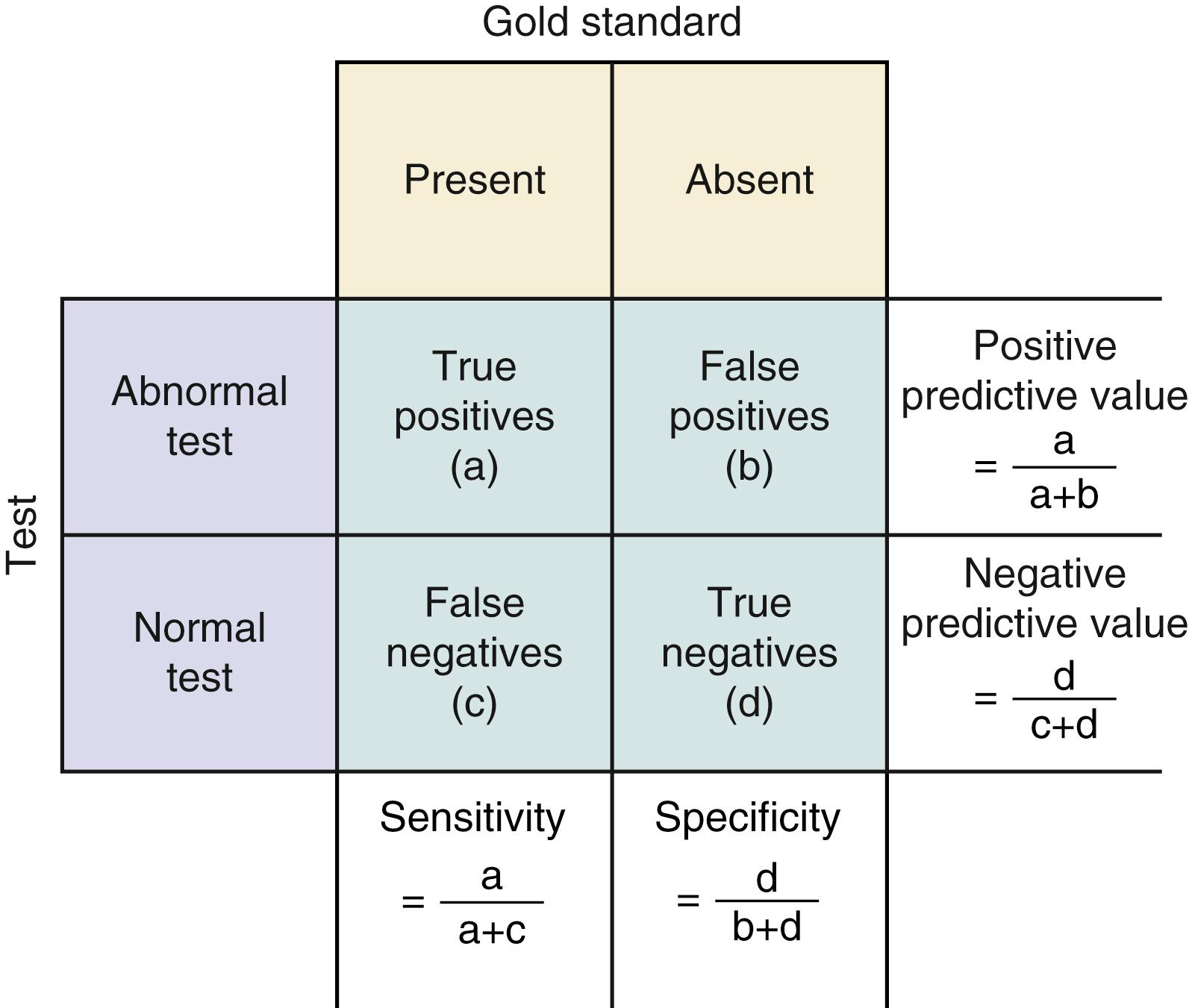
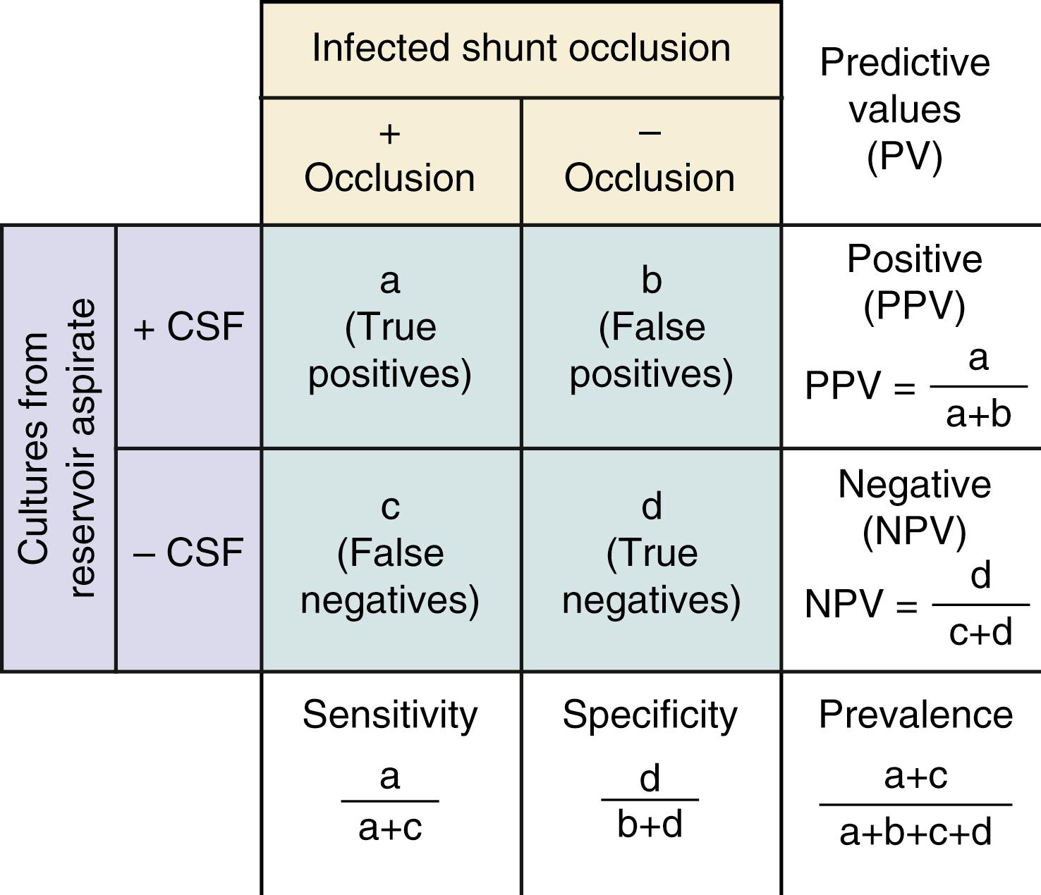
Sensitivity indicates the percentage of patients with a given illness who have a positive clinical finding or study. , In Fig. 76.3 , sensitivity is equal to a /( a + c ): If a patient has an infected shunt occlusion, how likely is it that the CSF aspirate from the reservoir will show a positive result? Conversely, specificity , equal to d /( b + d ) in Fig. 76.3 , refers to the proportion of patients without a clinical diagnosis who also do not have a clinical finding. If a patient does not have an infected shunt occlusion, how likely is it that the CSF aspirate will show a negative result?
If the sensitivity of a finding is very high (say, above 95%) and the disease is not overly common, then it is safe to assume that there will be few false-negative results (cell C in Fig. 76.3 will be small). Thus the absence of a finding with a high sensitivity for a given condition will tend to rule out the condition. When specificity is high, the number of false-positive results is low (cell B in Fig. 76.3 will be small) and the presence of a symptom will tend to rule in the condition. Epidemiologic texts have suggested that the mnemonics SnNout (when sensitivity is high, a negative CSF culture rules out an infected shunt occlusion) and SpPin (when specificity is high, a positive CSF culture rules in an infected shunt occlusion) be used, although some caution may be in order in applying these strictly.
However, when sensitivity or specificity is not as high or when a disease process is common, the more relevant clinical values are the number of patients with the symptom or study result who end up having the disease of interest, otherwise known as the positive predictive value (PPV = a /[ a + b ]). So if CSF cultures are positive, how likely is it that the patient has an infected shunt? The probability that a patient does not have the disease when the symptom or study result is absent or negative is referred to as the negative predictive value (NPV = d /[ c + d ]). Subtracting the NPV from 1 gives a useful “rule-out” value, providing the probability of a diagnosis even when the symptom is absent or the study result negative. If CSF culture results are negative, how likely is it that the patient is free of an infected shunt occlusion?
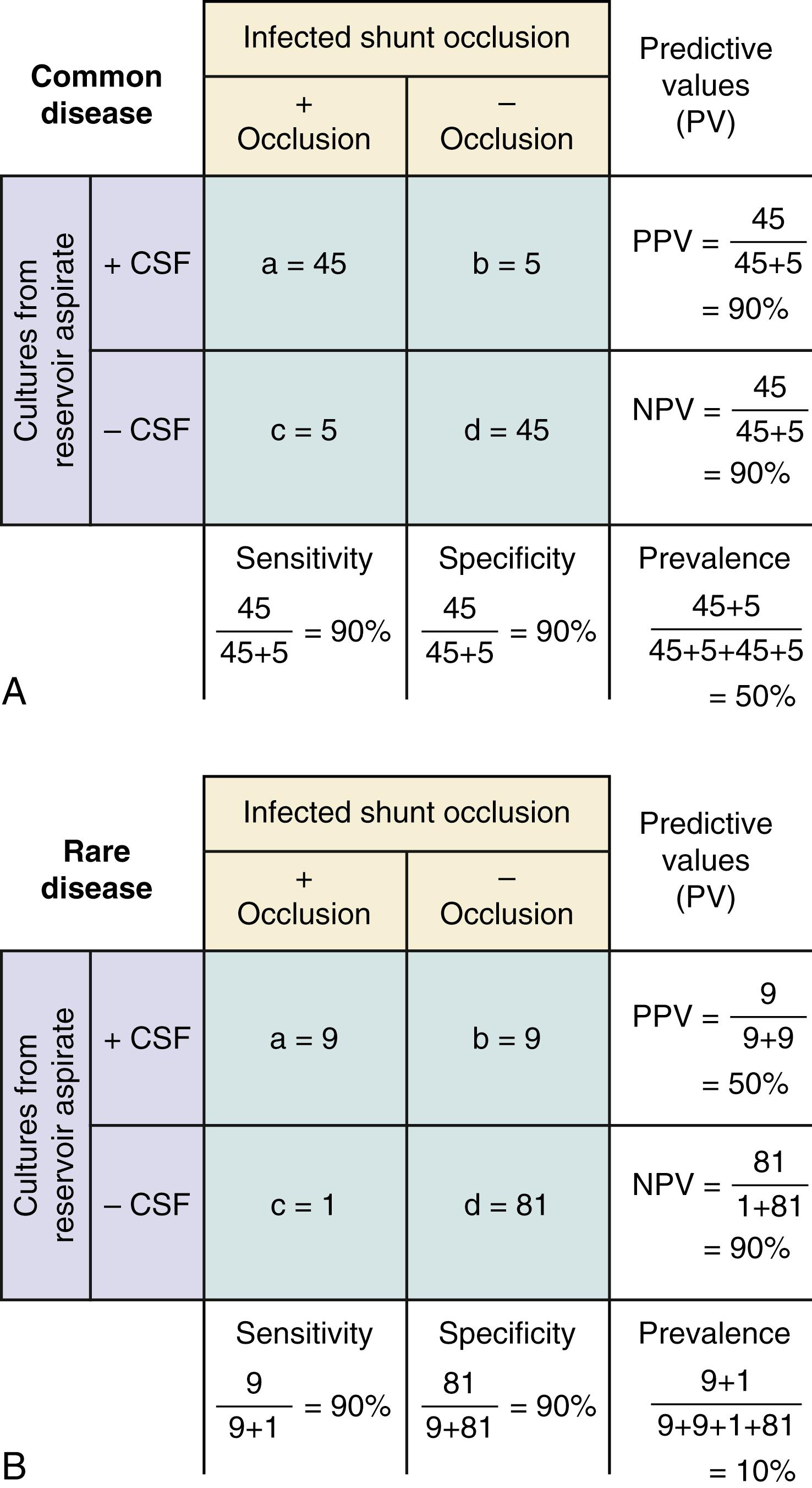
A key component of these latter two values is the underlying prevalence of the disease. Examine Fig. 76.4 . In both the common disease and rare disease cases, the sensitivity and specificity for the presence or absence of a particular sign are each 90%, but in the common disease case the total number of patients with the diagnosis is much larger, leading to higher PPVs and lower NPVs. When prevalence of the disease drops, the important change is the relative increase in the number of false- versus true-positive results, with the reverse true for false- versus true-negative results.
Likelihood ratios (LRs) are an extension of the aforementioned properties of diagnostic information. LRs express the odds (rather than the percentage) that a patient with a target disorder will have a particular finding present, as compared with the odds that the finding will be present in a patient without the target disorder. An LR of 4 indicates that it is four times as likely that a patient with an infected shunt occlusion will have a positive CSF culture, compared with patients without an infected shunt occlusion.
Reliability measures precision, or reproducibility, of a test. In Fig. 76.1 , note that the precision reflects the test’s ability to limit random error. In other words, reliability assesses variation, which may be broadly categorized into three types: intrasubject variation, intraobserver variation, and interoberver variation.
Intrasubject variation refers to variation within the individual subject. For example, measuring CSF flow from a puncture of the shunt reservoir varies depending on the position of the patient: supine, 30 degrees, upright, and so on. Limiting intrasubject variation here would entail standardizing the position of the patient.
Variation may occur between two or more readings from the same patient by the same observer. For example, after the CSF has been collected from the shunt tap, a neurosurgery provider may want to characterize the fluid collection as clear or cloudy. A single provider may label the same aliquot differently at two separate times, even though the CSF is the same and hasn’t changed between readings, with only the interpretation and designation of the observer having changed. Limiting intraobserver variation requires decreasing the subjective element, like measuring absorbance with a spectrophotometer in the lab.
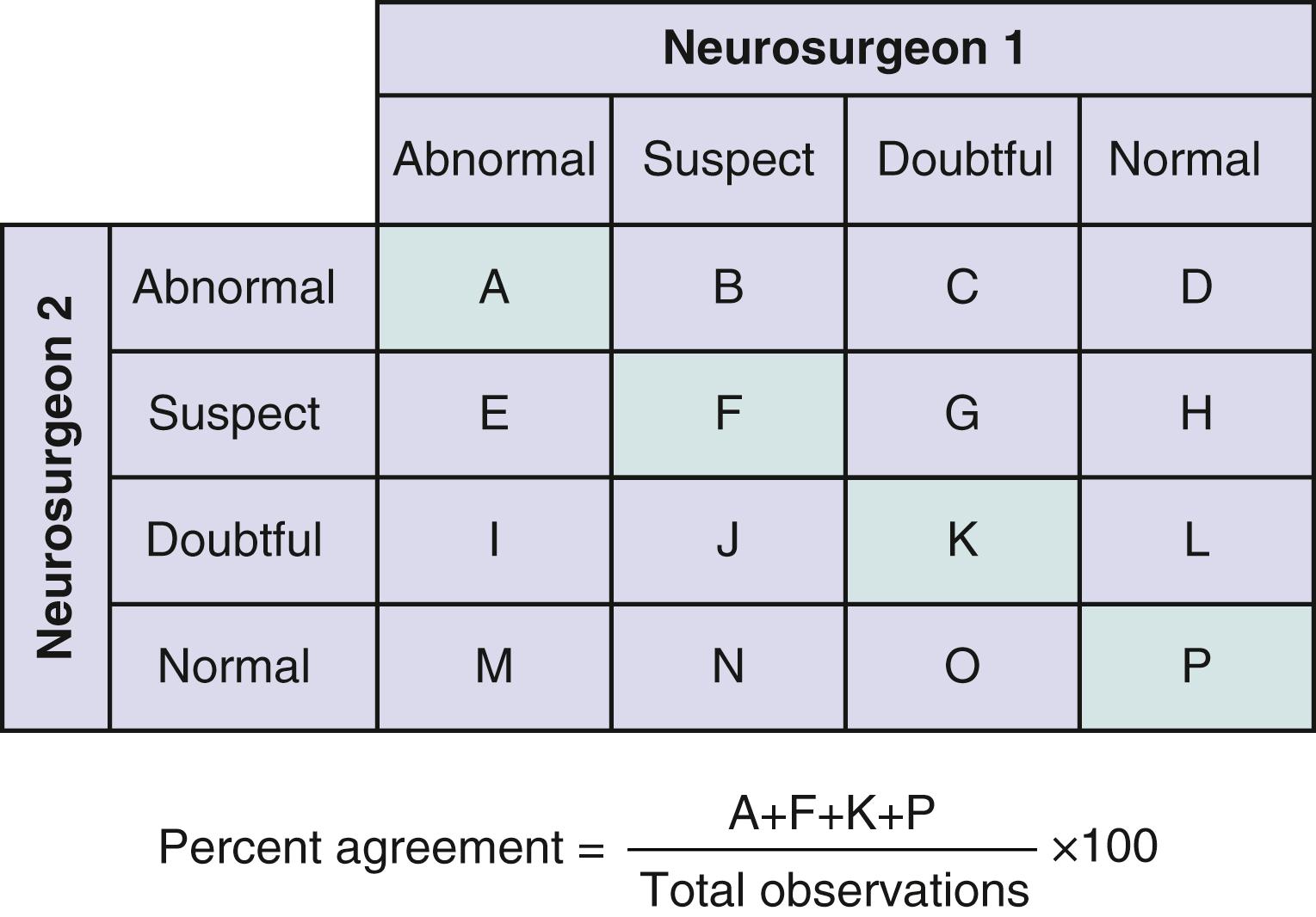
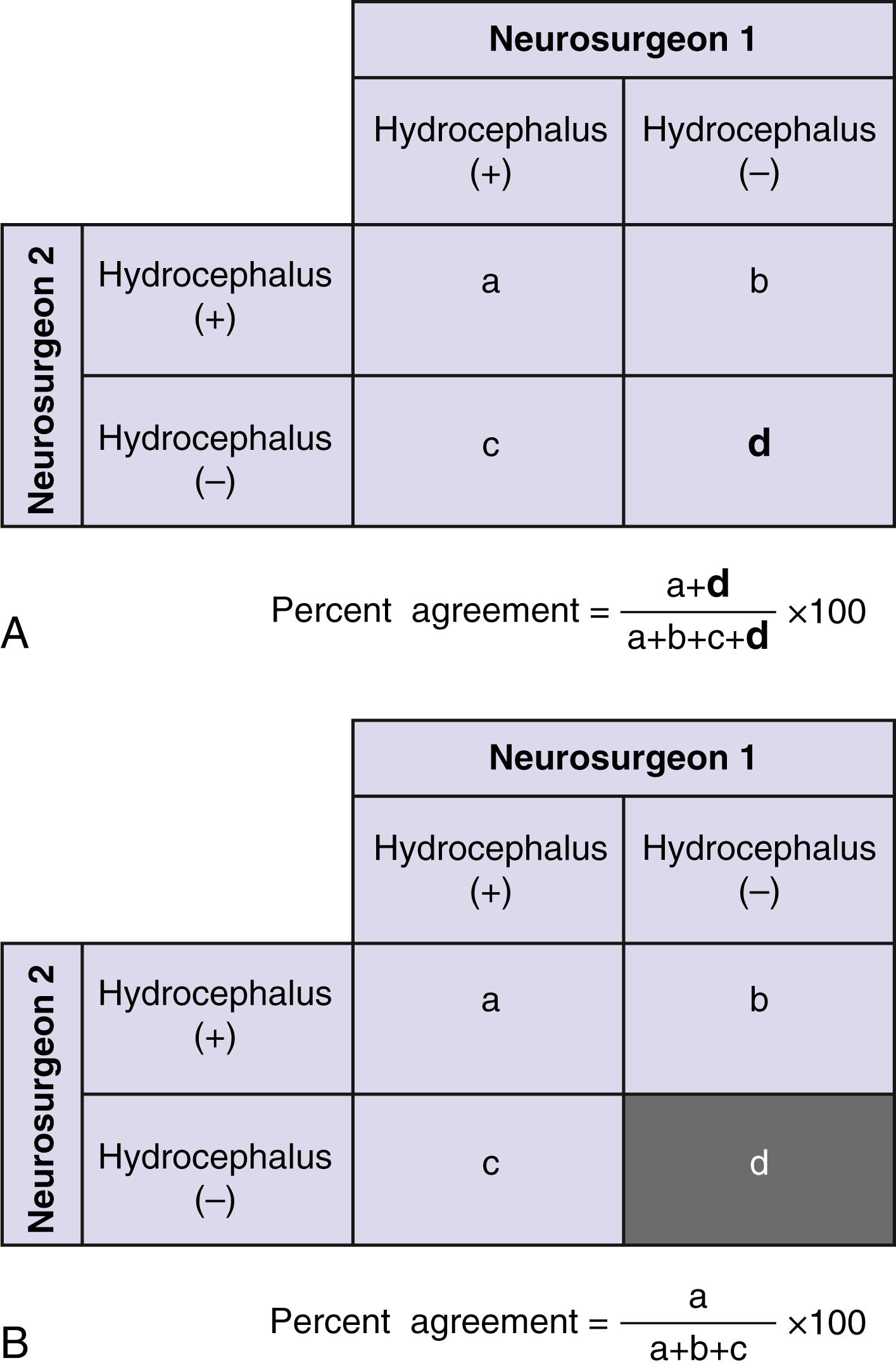
Variation between two observers is called interobserver reliability, which can be calculated as the percent agreement as seen in Figs. 76.5 and 76.6 . However, most patients will have negative results, for which observers will likely have considerable agreement. The percent agreement will subsequently become very high only because of the large number of clearly negative findings. This will conceal significant disagreement between observers for patients whose results are considered positive by at least one observer. This point can be best illustrated with a bayesian approach, similar to our analysis of validity in infected shunt occlusions. In Fig. 76.7 , two neurosurgeons are asked to report positive hydrocephalus versus negative hydrocephalus on non–contrast-enhanced CT among patients suspected to have infected shunt occlusions. By removing the number of patients who clearly do not have hydrocephalus on head CT, percent agreement on image findings becomes more meaningful.
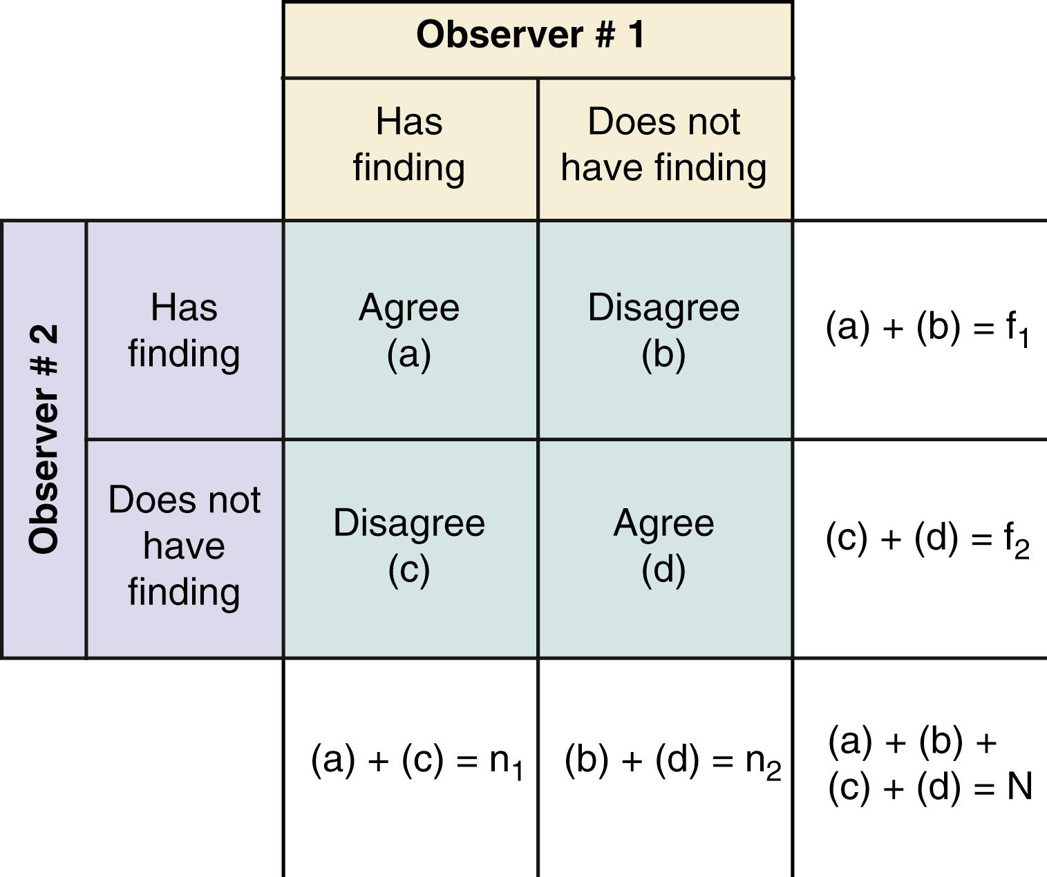
Percent agreement is only half of the narrative for interobserver variation. To what extent do two observers agree (e.g., two neurosurgeons evaluating hydrocephalus) beyond the agreement that would be expected by chance alone? The kappa statistic (κ)—commonly used for categorical data—numerically quantifies percent agreement beyond what would occur by chance.
An example of percent agreement for hydrocephalus between two independent neurosurgeons can be analyzed with a bayesian approach, seen in Fig. 76.8 . But how do we calculate percent agreement by chance alone? In Fig. 76.8 , suppose the first neurosurgeon always reports 60% positive hydrocephalus. Among 88 positive hydrocephalus scans read by the second neurosurgeon, the first neurosurgeon would find positive hydrocephalus in, at most, 60% (52.8 scans) by chance alone. Similarly, among the 62 negative hydrocephalus scans read by the second neurosurgeon, the first neurosurgeon will report negative hydrocephalus in, at most, 40% (24.8 scans) by chance alone. When these numbers are combined, percent agreement by chance alone equals 51.7%.
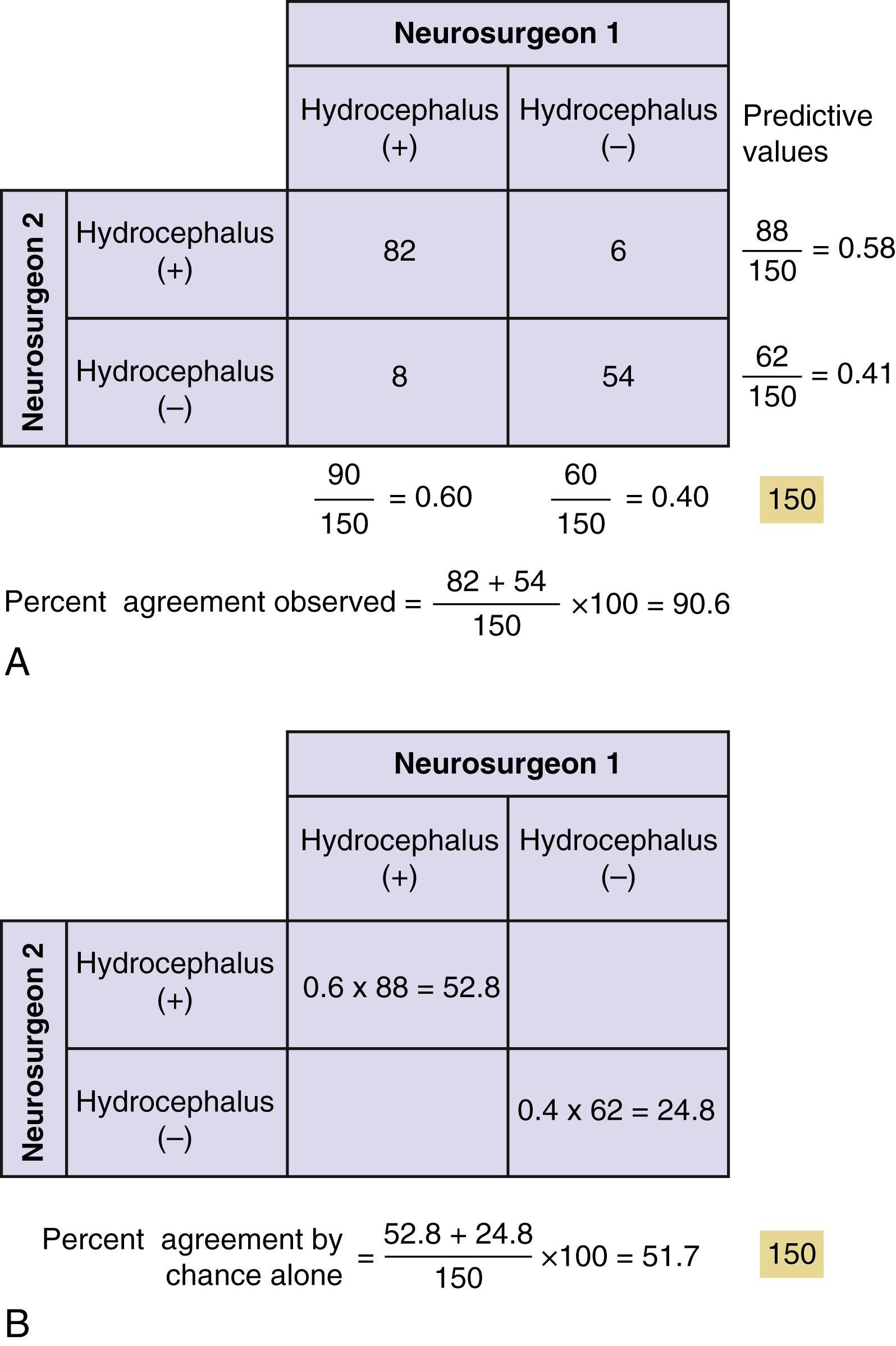
Interpretation of these κ values is somewhat arbitrary but, by convention, κ = 0 to 0.2 indicates slight agreement; κ = 0.2 to 0.4, fair agreement; κ = 0.4 to 0.6, moderate agreement; κ = 0.6 to 0.8, substantial agreement; and κ = 0.8 to 1.0, high agreement. So κ in our example shows only moderate agreement. Unlike previously described techniques to improve intrasubject variation or intraobserver variation, increasing the value of κ will require increasing the sample size, or the number of ratings. Therefore interobserver variation, a measure of precision or accuracy, is dependent on sample size. This becomes an important point when discussing power analyses later in the Biostatistics section.
In the prior section, the principles of screening testings or best intervention were discussed. Here, a different issue is addressed: How do we design a study to elucidate the risk factors or etiology of human disease?
Appropriate study designs sets the foundation for hypothesis-driven research that answers a meaningful question in neurosurgery. To better understand the features of study design, it is helpful to consider factors that limit the ability of a study to answer that question. In this context, it is easier to understand the various permutations of clinical research design. Different study designs are more or less robust in managing the various study biases or opportunities for error that must be considered as threats to their validity ( Tables 76.1 and 76.2 ).
| Example | Limitations (Typical) | |
|---|---|---|
| Descriptive Studies | ||
| Population correlation studies | Rate of disease in population vs incidence of exposure in population | No link at the individual level, cannot assess or control for other variables; used for hypothesis generation only |
| Changes in disease rates over time | No control for changes in detection techniques | |
| Individuals | ||
| Case reports and case series | Identification of rare events, report of outcome of particular therapy | No specific control group or effort to control for selection biases |
| Cross-sectional surveys | Prevalence of disease in sample, assessment of coincidence of risk factor and disease at a single point in time at an individual level | “Snapshot” view does not allow assessment of causation, cannot assess incident vs prevalent cases; sample determines degree to which findings can be generalized |
| Descriptive cohort studies | Describes outcome over time for specific group of individuals, without comparison for treatments | Cannot determine causation; risks of sample-related biases |
| Analytical Studies | ||
| Observational | ||
| Case control studies | Disease state determined first Identified control group retrospectively compared with cases for presence of particular risk factor |
Highly subject to bias in selection of control group; generally can study only one or two risk factors |
| Retrospective cohort studies | Population of interest determined first, outcome and exposure determined retrospectively | Uneven search for exposure and outcome between the groups; susceptible to missing data; results dependent on entry criteria for cohort |
| Prospective cohort studies | Exposure status determined in a population of interest, then followed for outcome | Losses to follow-up over time, expensive, dependent on entry criteria for cohort |
| Interventional | ||
| Dose escalation studies (phase I) | Risk of injury from dose escalation | Comparison is between doses, not vs placebo; determines toxicity not efficacy |
| Controlled nonrandomized studies | Allocation to different treatment groups by patient/clinician choice | Selection bias in allocation between treatment groups |
| Randomized controlled trials | Random allocation of eligible subjects to treatment groups | Expensive; experimental design can limit generalizability of results |
| Meta-analyses | Groups randomized trials together to determine average response to treatment | Limited by quality of original studies; difficulty combining different outcome measures; variability in base study protocols |
| Bias Name | Explanation |
|---|---|
| Sampling Biases | |
| Prevalence-incidence | Drawing a sample of patients late in a disease process excludes those who have died from the disease early in its course. Prevalent (existing) cases may not reflect the natural history of incident (newly diagnosed) cases. |
| Unmasking | In studies looking at causation, factors that cause symptoms may be sought, which in turn cause a more diligent search for the disease of interest. Example might be if a particular medication caused headaches and this led to the performance of more MRIs, leading to an increase in the diagnosis of arachnoid cyst among patients taking the medication. The conclusion that the medication caused the arachnoid cyst would reflect unmasking bias. |
| Diagnostic suspicion | A predisposition to consider an exposure as causative prompts a more thorough search for the presence of the outcome of interest. |
| Referral filter | Patients referred to tertiary care centers are often not reflective of the population as a whole, in terms of disease severity and comorbidities. Natural history studies are particularly prone to biases of this sort. |
| Chronologic | Patients cared for in previous time periods likely received different diagnostic studies and treatments. Studies with historical controls are at risk. |
| Nonrespondent/volunteer | Patients who choose to respond or not respond to surveys or follow-up assessments differ in tangible ways. Studies with incomplete follow-up or poor response rates are prone to this bias. |
| Membership bias | Cases or controls drawn from specific self-selected groups often differ from the general population. The result of this bias is the assumption that the group’s defining characteristic is the cause of the group’s performance with respect to a risk factor. |
| Intervention Biases | |
| Cointervention | Patients in an experimental or control group systematically undergo an additional treatment, not intended by the study protocol. If a treatment were significantly more painful than a control procedure, a potential cointervention would be the increased analgesic use postoperatively. A difference in outcome could be due either to the treatment or to the cointervention. |
| Contamination | When patients in the control group receive the experimental treatment, the potential differences between the groups are masked. |
| Therapeutic personality | In unblinded studies, the belief in a particular therapy may influence the way in which provider and patient interact, altering outcome. |
| Measurement Biases | |
| Expectation | Prior expectations about the results of an assessment can substitute for actual measurement. In assessments of either diagnosis or therapy, belief in the predictive ability or the therapeutic efficacy increases the likelihood that a positive effect will be measured. Unblinded studies and those with subjective outcome measure are prone to this bias. |
| Recall | In cohort and case-control studies, different assessment techniques or frequencies applied to those with the outcome of interest may increase the likelihood of detection of a risk factor—in particular, asking cases multiple times vs controls improves chances for recall. This especially applies to retrospective studies and is the inverse of the diagnostic suspicion bias above. |
| Unacceptability | Measurements that are uncomfortable, either physically or mentally, may be avoided by study subjects. |
| Unpublished scales | The use of unpublished outcome scales has been shown in certain settings to result in a greater probability of the study finding in favor of experimental treatment. |
| Analysis Biases | |
| Post hoc significance | When decisions regarding levels of significance or statistical measures to be used are determined after the results have been analyzed, it is more likely that a significant result will be found. It is very unlikely that authors would state this in a manuscript, but protection is afforded by publication of the study methods in advance of the study itself. |
| Data dredging | Multiple questions of a data set are asked until something with statistical significance is found. Subgroup analysis, depending on whether preplanned and coherent with the study aims and hypotheses, may also fall into this category. |
Common in the neurosurgical literature, case reports describe a single patient, whereas case series describes a group of patients. These studies properly have their place in describing new or unusual medical events. In such studies, there is an implicit comparison with what is usual or ordinary in clinical practice. They can suggest possible causes and treatments for events but can offer only limited support for clinical practice patterns and do not allow for hypothesis testing, but can be useful in hypothesis generation. The main attraction of these types of studies is that they are easy and inexpensive to complete. They can also provide data important in designing subsequent, more complex investigations, particularly if standard outcome measures are used in the analysis. This type of study can be considered prognosis (natural history) or “prognosis with treatment” studies, depending on the research study question or hypothesis. An example in CSF shunt infection would be looking at patients with this diagnosis and seeing how various treatments were successful.
Cross-sectional studies attempt to determine the presence of disease and potential exposures or risk factors causing the disease in individuals at a single point in time. Often based on interviews or questionnaires, or medical chart reviews, such studies can usually be accomplished relatively inexpensively and quickly in comparison to the comparative cohort studies they mimic. The principal limitation is that because the data are collected at a single point in time, they cannot be used to determine the causal relationship between an exposure and the disease of interest. In addition, the single time assessment does not allow for understanding of the course of illness. Thus cross-sectional studies establish the prevalence of any given variable, not the incidence.
Cohort studies are primarily used to assess the role of common exposures with modest effects on disease incidence or progression. They can help to establish an appropriate temporal relationship between exposure and outcome, and can simultaneously investigate a number of potential risk factors for a disease outcome. In the traditional cohort study, investigators assemble a large group of individuals. This group is then assessed for a variety of exposures and followed, usually with serial assessments over time to determine the subsequent occurrence of outcome events. Drawing all of the members of the cohort from the same setting is one of the ways in which studies of this type try to minimize selection bias. Keys to the study design include a constant method of assessment for all members of the cohort regardless of potential exposure, and complete follow-up.
In prospective cohort studies, the outcome events are unknown at the time the study is started and patients are followed into the future. In retrospective cohort studies, the investigator is looking backward to determine the exposure history for the cohort after the outcome is already known. As always, the prospective study is more robust methodologically, as it offers much better protection against assessment biases for the exposure. Retrospective studies are at risk for diagnostic-suspicion bias —investigating those with the outcome of interest more closely than those without and thus lending bias to the reported relative risks. Prospective studies, however, face a greater problem with losses to follow-up.
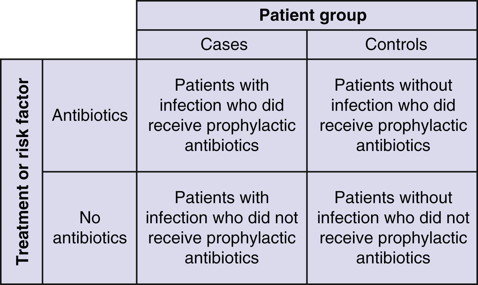
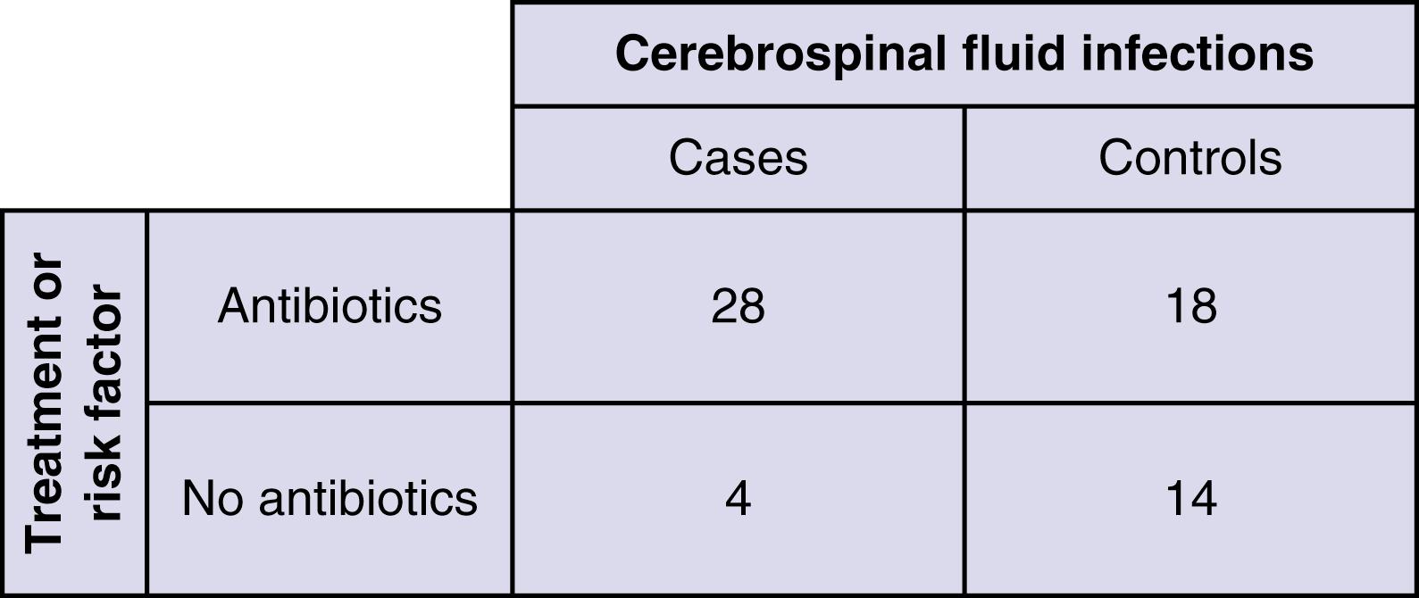
Performed retrospectively, the case-control study starts with outcomes of interest rather than treatment, selecting a control group of patients who can then be compared with the cases with the chosen outcome ( Fig. 76.9 ). Originally designed to assess causation in rare diseases wherein a cohort would have to be prohibitively large to detect enough cases, the relative simplicity and easy retrospective application of this methodology have made for its widespread use. Patients with the disease or outcome of interest are identified first. Then a control population not showing the disease or outcome of interest is determined, and the two groups are assessed for the presence of particular risk factors. The result is typically an odds ratio of the risk factor in the cases versus the controls. Controls must be selected such that if they had developed the disease, they would have been eligible to be cases. Controls may be selected at random from a sample, but because such studies are usually small in total number, it is generally important to balance or match the cases and controls for important prognostic factors so that these do not obscure associations between the outcome and the factors of interest. From the standpoint of bias, case-control studies are most susceptible in the choice and assignment of the control patients and in the way in which the two groups are screened for the presence of risk factors. Controls should be contemporary to cases; if they are “historical,” they are open to a chronology bias, based on changes in practice patterns and the influence of changing technology over time. It is important to understand that case-control studies can also be used in the scenario of treatment as well as causation. For example, when trying to decide whether to use prophylactic antibiotics to prevent shunt infection, cases can be compared with controls to determine what the frequency of antibiotic use was in the two groups ( Fig. 76.10 ). Comparison of categorical data can then be performed with a Fisher exact test.
Become a Clinical Tree membership for Full access and enjoy Unlimited articles
If you are a member. Log in here