Laboratory Statistics

Definitions

• Variables: The things that we measure, count, or otherwise delineate are termed variables because the values they can assume vary. Variables are usually considered to fall into one of the following scales.

• Nominal scale is where a variable can take on only a limited number of values, usually called categories (or characters ). Examples of nominal variables are gender (male or female) and risk factors (e.g., smoker or nonsmoker).

• Ordinal scale is where the variable takes on specific values that have some inherent order, such as magnitude but without equivalent distances between categories (e.g., trace amount, 1+, 2+, etc., of protein in urine).

• Interval scale is where a variable takes on values in a quantitative range with defined differences between points. It is conventional to treat most numeric laboratory measurements as continuous variables, even though they may be reported as discrete values (e.g., glucose values of 123 or 124 mg/dL, but not 123.857… mg/dL).

• Coefficient of variation (CV) is the standard deviation of a set of data points divided by the mean result expressed as a percentage or as a decimal fraction.

• Confidence interval (CI) is the interval that is computed to include a parameter such as the mean with a stated probability (e.g., commonly 90%, 95%, 99%) that the true value falls into that interval.

• Degrees of freedom (df) is a parameter related to the sample size (n). df indicates the number of quantities free to vary and is usually n − 1 for applications such as the t -test. For the chi-square test, it is the number of rows minus one times the number of columns minus one. df is employed in calculating the p value for a statistical test.

• Gaussian (normal) distribution is a spread of data in which elements are distributed symmetrically around the mean, with most values close to the center. It is explicitly described by a mathematical equation, as is a parametric distribution. Random scatter or random selection of a population often results in a Gaussian normal distribution. This type of distribution is often a criterion for completely valid application of many parametric tests.

• Linear regression is the mathematical process for calculating the best straight line to fit the relationship observed between two variables measured on the same items. Simple or least squares linear regression yields the best fit for x and y data sets by minimizing the sum of the squared y -axis (vertical distance) differences between each data point (x, y) and the line. This approach assumes the x -axis data to be nearly perfect or without error. Uneven distribution of data points across the entire range may significantly alter the reliability of linear regression. Deming linear regression does not assume the x -axis data to be free of error, but instead uses the weighted sum of squared y -axis and x -axis differences between the data points and the line. The correlation coefficient (r) describes how well the line fits the data ( r ranges from −1 to 1).

• Mean is the sum of all results divided by the number of results. Also related are the median, which is the middle value that divides the distribution of data points into upper and lower halves (also called the 50th percentile), and the mode , which is the most common value. The mean, median, and mode are all measures of central tendency. The geometric mean is calculated as the n th root of the product of a distribution of n numbers; its use for estimating central tendency minimizes the effects from extreme values such as are found in a log-normal distribution.

• Parametric statistics are statistical measures that are calculated based on the assumption that the data points follow a Gaussian distribution and include parameters such as mean, variance, and standard deviation. Nonparametric statistics are based on rank or order of data.

• Null hypothesis (H ₀ ) is the proposal that there is no difference in a comparison. The alternative hypothesis is that there is a difference. When the critical value of a statistic is exceeded, rejection of the null hypothesis occurs, thereby favoring the acceptability of the alternative hypothesis.

• Significance level (p or α) is the probability that a difference between groups occurred by chance alone, by convention set at less than 0.05.

• Statistical power (1 − β) is the probability that a difference between groups will be detected by the study, generally set to at least 80%.

• Standard deviation (SD) is the square root of the sum of the squared differences of each data point from the mean divided by n − 1 for samples (divided by n for populations). The SD is a predictable measure of dispersion from the mean in a Gaussian normal distribution.

• Standard deviation index (SDI) is the difference between the value of a data point and the mean value divided by the group’s SD. The z-transformation is the expression of a result from the mean in SD units. The Z -value is the probability of a result being z SDs from the mean value. The SDI is commonly used in reporting performance in proficiency testing for an individual laboratory compared with peers.

• Student t- test is a statistical test for comparing means between two sample groups. The test can be paired (e.g., two separate measurements on the same individuals before and after some intervention) or unpaired. Values of t and df yield a level of statistical significance ( p value).

• Type I error (alpha error, α) is incorrectly rejecting the null hypothesis and stating that two groups are statistically different when they really are not.

• Type II error (beta error, β) is incorrectly failing to reject the null hypothesis and stating that two groups are not statistically different when they really are.

Variables

Statistical questions are often posed in terms of input versus output, cause and effect, or correlation between two or more variables. The input or cause is considered an independent variable because it is already determined and therefore is not influenced by other factors. Examples of independent variables are age, gender, temperature, and time. In contrast, dependent variables are those things that might change in response to the independent variable. Examples of dependent variables are blood glucose concentration, enzyme activities, and the presence or absence of malignancy. Of course, we can change our thinking and switch which is the independent and which is the dependent variable if the experimental question changes. For graphical display, the independent variable is plotted along the horizontal (x) axis or abscissa, while dependent variables are plotted along the vertical (y) axis or ordinate. With a single independent variable (e.g., time) on the x -axis, more than one dependent variable can be plotted on the y -axis to demonstrate different relationships simultaneously. The relationship observed between an independent variable and dependent variables is used to predict future outcomes of the dependent ones based on what values the independent variable assumes.

Preparing to Analyze Data

Most statistical calculations today are done automatically by computer with software programs that present multiple sophisticated options for analysis and even graphical displays of the data. To prepare data for these automated analyses, it is always necessary to enter them into readable format for the program. This process can entail automated transfer from one electronic data set to the statistical program or manual entry from printed sheets of data. Manual entry is obviously fraught with opportunity for typographic errors, but even automated transfer of data can result in erroneous entries, especially when translating older data sets that have been stored on media that might have been corrupted (e.g., magnetic tapes reexamined decades later). Even converting data strings to columns and rows of data points can leave some values in the wrong places. Consequently, it is always good practice to examine the data set for accuracy before performing the statistical analysis. This examination could be done by proofreading every entry or by double entry of each value and automatic comparison for discrepancies, although both of these approaches may be impractical when the data sets contain hundreds, thousands, or more values. At the very least, visual examination of the plotted values provides a quick idea of whether some serious data entry errors have occurred. For example, an incorrectly entered value of 50.0 for potassium (instead of 5.0) can be immediately identified by scanning all values on a graphic plot. The person preparing to perform statistical analyses should do this visual test to identify and correct the most obvious errors and to search for any systematic errors that might have arisen in data transfer and entry.

Descriptive Statistics

When multiple data points are collected, it is useful to provide a summary of those results that makes them easier to understand rather than simply listing all values. The methods used to summarize data are termed descriptive statistics because they describe what the magnitude of results is and how the data points differ from one another. In the case of categorical variables, this description can be a simple count of discrete values (e.g., how many men and how many women had blood drawn in a clinic). For continuous variables, it is conventional to use some measure of central tendency about which the data points cluster and a measure of how far apart they are dispersed from one another (e.g., the ages of the patients who had blood drawn).

Gaussian (Normal) Distribution

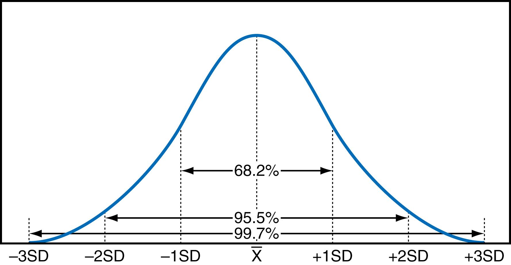
The Gaussian (also called normal ) distribution is a symmetric, bell-shaped curve centered about the mean value ( Fig. 10.1 ). It is described by the following mathematical formula:

$\text{P}\left(\text{x}\right)=\frac{1}{\text{σ}\sqrt{\text{π}}}{\text{e}}^{-\left(\frac{{\left(\text{x}-\overline{\text{x}}\right)}^2}{2{\text{σ}}^2}\right)},$

where σ is the standard deviation of the ideal Gaussian population ( ). It corresponds to the distance from the mean to the x value at which the curve has an inflection point.

The area under this curve within ±1 σ from the mean is approximately 68.2% of the total area, meaning that 68.2% of data points from a Gaussian distribution should fall within ±1 σ of the mean. Similarly, 95.5% of the data points will be within ±2 σ of the mean, and 99.7% will be within ±3 σ of the mean.

Dispersion

A common parametric measure (based on the Gaussian distribution) of the dispersion of data points about the mean value of a population under examination is the standard deviation, mathematically calculated as:

$\text{SD}=\sqrt{\frac{{\sum }_{\text{i}=1}^{\text{n}}{\left({\text{x}}_{\text{i}}-\overline{\text{x}}\right)}^2}{\text{n}-1}}$

The quantity under the square root sign is termed the variance . Use of the SD assumes that the data follow a bell-shaped curve that can be described mathematically by the formula for a normal or Gaussian distribution. To the extent that the data are normally distributed, the SD is a good estimate of the dispersion.

Two additional terms derive from the SD. One is the coefficient of variation (CV) , which is calculated as the SD divided by the mean. The CV is often expressed as a percentage, although it can also be expressed as a decimal fraction less than 1. For a situation in which the mean = 25 and the SD = 5, the CV = 20%, or 0.20. The other term is the standard deviation index (SDI) , which is the distance that an individual data point is away from the mean value divided by the SD. The main use for the SDI is in such applications as proficiency testing, where performance of any one laboratory is standardized according to the dispersion of data in the performance by all laboratories.

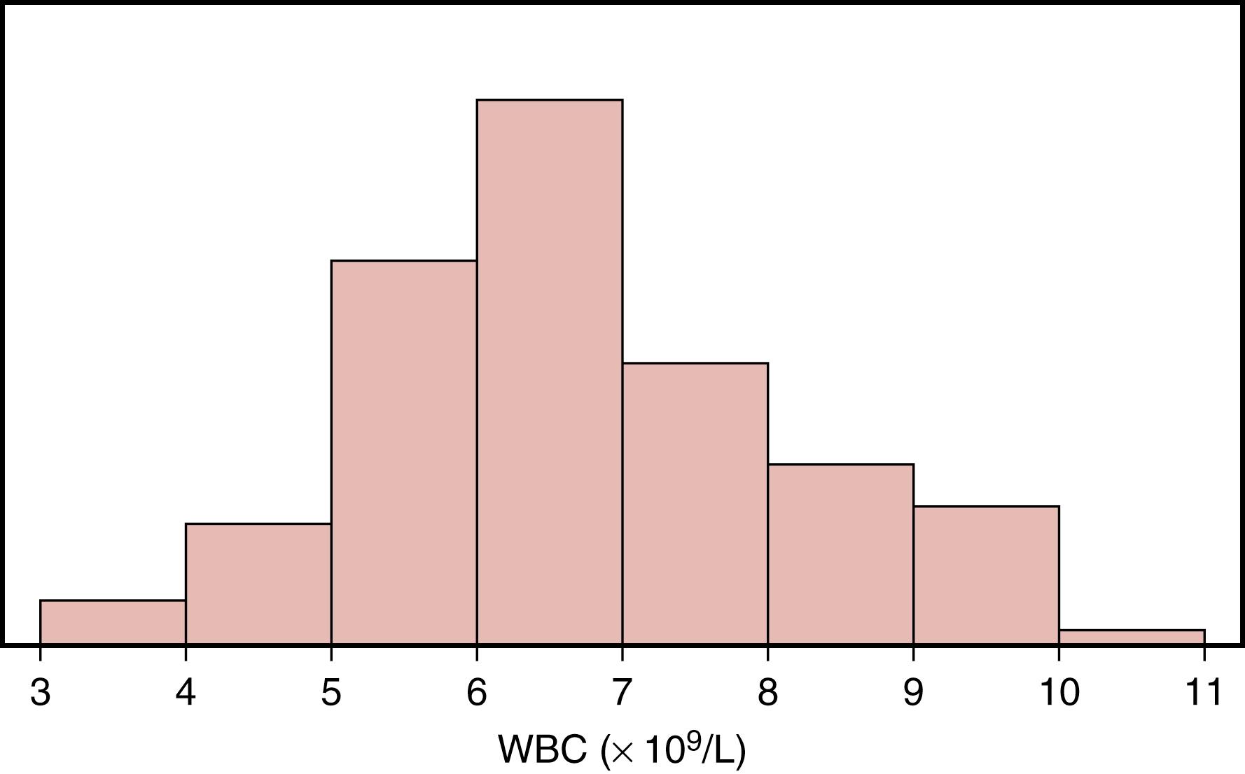
A common clinical laboratory application of the normal distribution is to calculate the central 95% of values obtained from a healthy population when trying to establish the reference range for an analyte. This range, of course, is easily calculated as mean ±2 SD for a truly Gaussian normal population. An example of this application is calculation of the central 95% of values of the white blood cell (WBC) count in a group of 85 healthy medical students ( Fig. 10.2 ). The bar graph plot is roughly bell-shaped and symmetric, although there is a slight asymmetry that can probably be ignored. The mean value is 6.60 × 10 ⁹ cells/L, with an SD of 1.457 × 10 ⁹ cells/L, and the calculated central 95% range is from 3.69 to 9.52 × 10 ⁹ cells/L. This is a small group of individuals compared with what might be used for actual reference range calculations, but it does show a few persons with WBCs higher than this range and some lower. Thus, this estimate of central 95% appears appropriate.

Another way of thinking about these calculations is that the persons tested represent only a sample of all persons to whom we are interested in generalizing these findings ( ). The mean value actually observed would probably be somewhat different if another group of 85 healthy people were tested. Based on the values observed and their spread, a confidence interval can be placed around the mean such that we can be certain by a desired percent that the true mean of WBCs from all healthy persons falls in that range. The confidence limit is calculated as follows:

$\text{Confidence interval}=\overline{\text{x}}\pm \text{z}\frac{\text{SD}}{\sqrt{\text{n}}},$

where the critical factor z derives from transformation of the problem to a standard normal distribution. The quantity $\frac{\text{SD}}{\sqrt{\text{n}}}$ is termed the standard error of the mean . In this example, let the confidence interval be 95%, for which z = 1.96. The 95% confidence interval around the mean value is:

$6.60\pm 1.96\times \frac{1.457}{\sqrt{85}}\text{or}6.295-6.914\times {10}^9\text{cells}/\text{L}\text{.}$

Note that this range is the 95% confidence interval on the mean value alone, whereas the earlier calculations yielded the central 95% of all data points. Confidence intervals are used to give an idea of the broadness of the estimate of something. This can be made more certain by using 99% confidence intervals (i.e., 99% confident that the true mean falls in the interval), in which case z = 2.575 for the calculation, and the 99% confidence interval is broader at:

$6.60\pm 2.575\times \frac{1.457}{\sqrt{85}}\text{or}6.193-7.007\times {10}^9\text{cells}/\text{L}.$

Nonparametric Measures

The median value of WBCs for this group of healthy persons is 6.4 × 10 ⁹ cells/L, which is roughly the same as the mean value. For a perfectly Gaussian normal distribution, values of the mean, median, and mode are exactly the same. Delineation of the range from the 2.5-percentile to the 97.5-percentile also gives an estimate of the central 95% range (for the example of WBCs, it is 3.94 to 9.89 × 10 ⁹ cells/L, which is really the exact range for this specific population). This is a nonparametric estimate of the range because it does not use a calculation but rather divides the data points only according to their order. Many applications of median use the central 50% of data points from the 25th percentile to the 75th percentile (also called interquartile range) to describe central tendency by the nonparametric method.

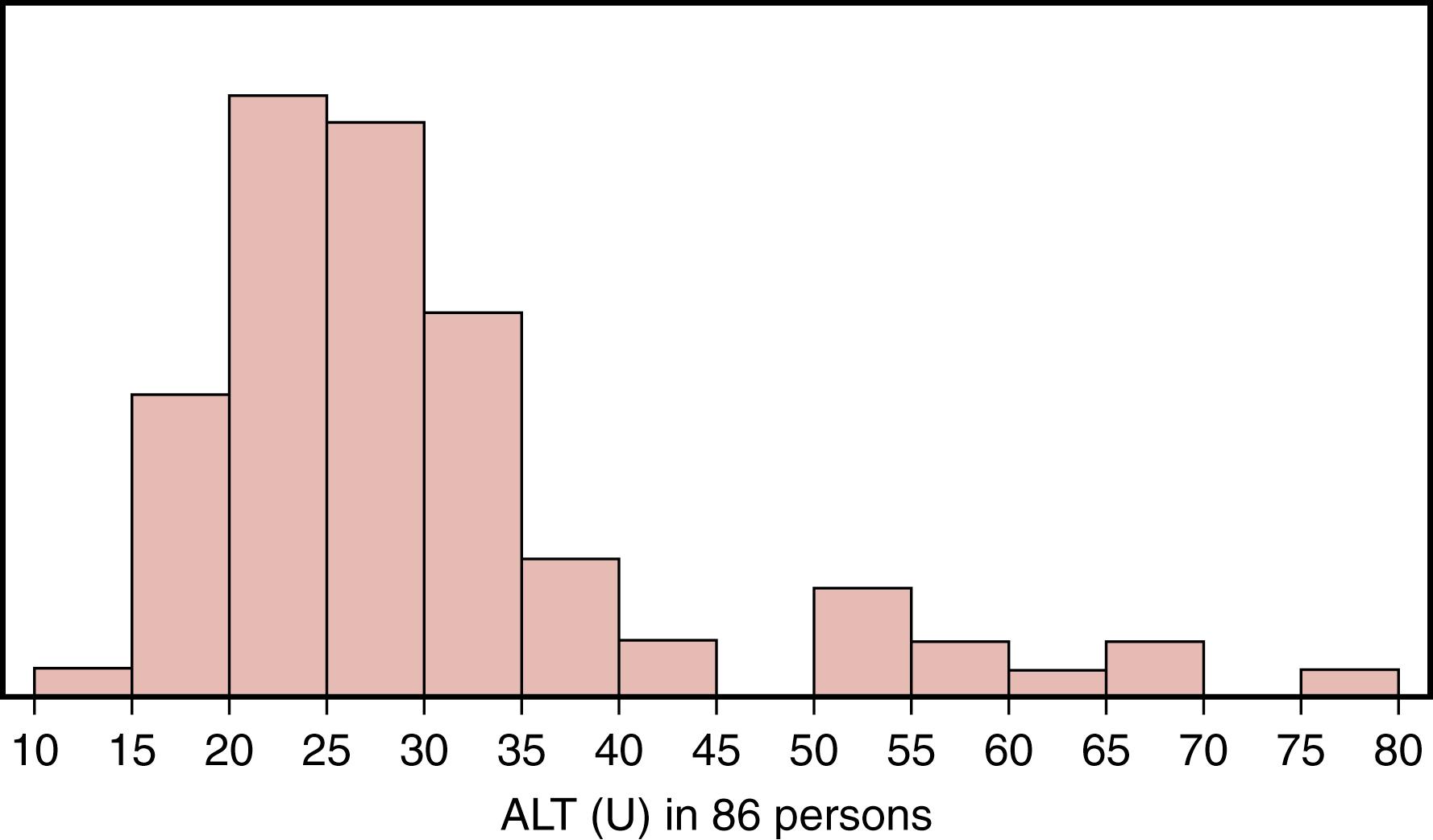
Sometimes, the parametric method of mean ±2 SD produces an erroneous estimate of the central 95% range. An example of this situation arises with the distribution of alanine aminotransferase (ALT) activities in the serum of apparently healthy individuals ( Fig. 10.3 ). In this population, the mean value is 30.1 U, the SD is 12.69 U, and the calculated reference range (mean ±2 SD) is 4.73 to 55.48 U. This range is not appropriate because the actual lowest value observed in the group was much higher (12 U). This estimate of the lower end of the range (4.73 U) is far too low. Similarly, the estimate of the upper end (55.48 U) is too low and excludes about 10% of the data points instead of only 2.5%. Another clue that the parametric method may not work here is that the median value is 27.0 U, which is somewhat different from the mean. The reason for this discrepancy is apparent upon looking at the distribution, which is skewed to the right with many values tailing off at the upper end. In this case, a much more useful estimate of the central 95% can be obtained simply from the 2.5-percentile to the 97.5-percentile range. It is 15.2 to 68.0 U. The form of this distribution for ALT is sometimes termed log-normal , because it can be converted to a normal distribution by using the values of log ALT instead.

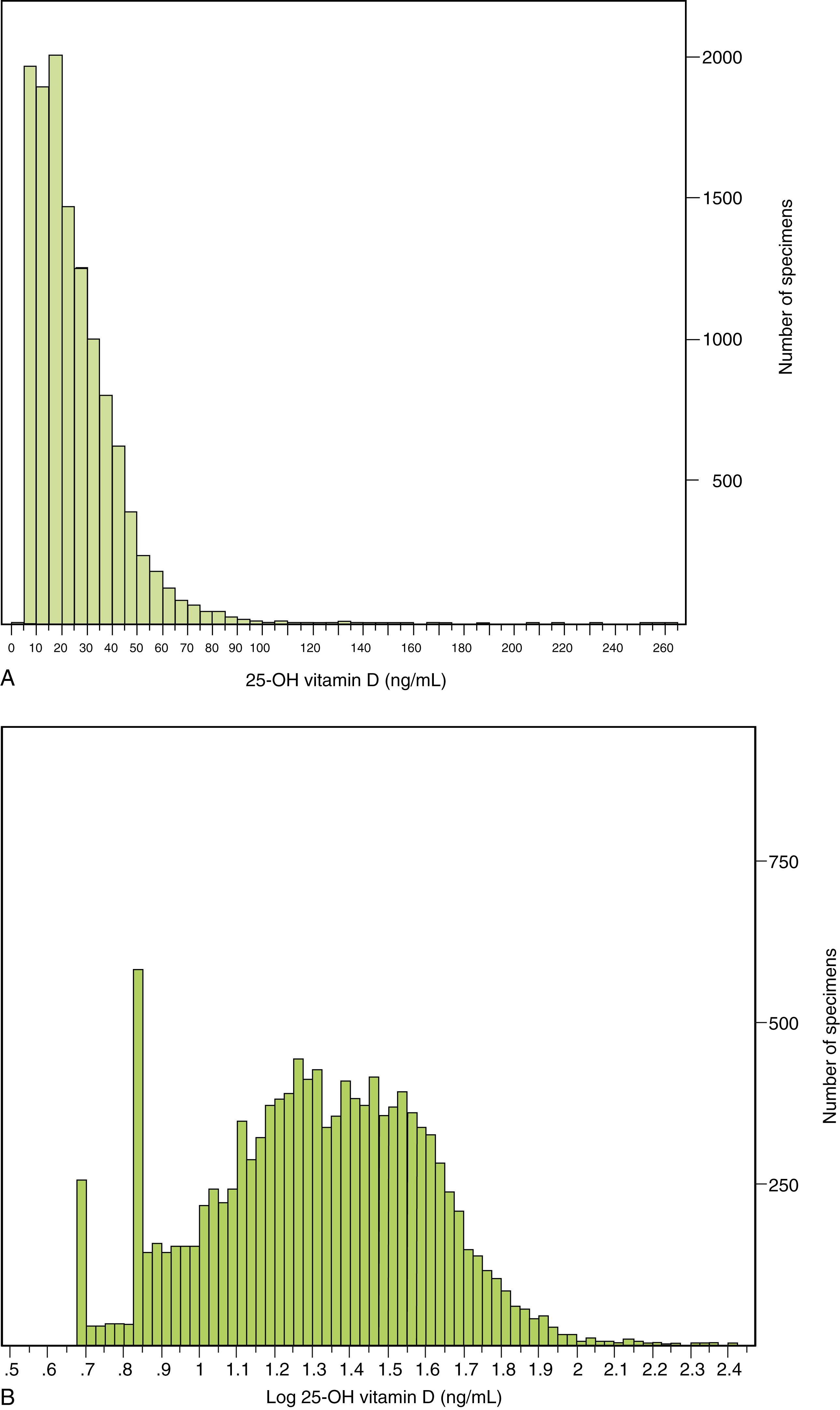
Many laboratory measurements show distinctly non-Gaussian normal distributions. Values of 25-OH vitamin D in 12,434 serum specimens from 2000 through 2008 showed a skewed distribution, with lowest value 0.5 ng/mL and highest value 260.0 ng/mL ( Fig. 10.4A ). The arithmetic mean of these values is 25.55 ng/mL, and the median is 20.90 ng/mL, reflecting the nonnormal distribution. Plotting log 25-OH vitamin D shows a nearly normal distribution with mean value 1.3130 ( Fig. 10.4B ). Then, the geometric mean is 10 ^1.3130 = 20.56 ng/mL, which appears to be a better measure of central tendency for 25-OH vitamin D than the arithmetic mean.

Comparative Statistics

One of the questions frequently asked by statistical means is whether one group is different from another group in some characteristic. The question boils down to a comparison of the central tendency of one group versus that of the other and the scatter that each group exhibits about the central values. If the scatter of data is extreme, then calculated differences between mean values of two groups might not be important but rather the result of adding in the extreme values. Another way to think about these comparisons is that of signal/noise ratio. If there is little noise (scatter of data), then the difference in the signal from each group is more believable.