Basic Statistics for Electrodiagnostic Studies

For every electrodiagnostic (EDX) test performed, one needs to decide if the study is normal or abnormal. That determination often needs to be made in real time as the testing progresses, so that the study can be modified based on new information obtained as the testing proceeds. However, interpreting a test as normal or abnormal is not always straightforward and requires some understanding of basic statistics. A full discussion of statistics is beyond the scope and purpose of this text, but there are some basic statistical concepts that every electromyographer needs to know to properly interpret a study.

No two normal individuals have precisely the same findings on any biologic measurement, regardless of whether it is a serum sodium level, a hematocrit level, or a distal median motor latency. Most populations can be modeled as a normal distribution , wherein there is a variation of values above and below the mean. This normal distribution results in the commonly described bell-shaped curve ( Fig. 9.1 ). The center of the bell-shaped curve is the mean or average value of a test. It is defined as follows:

Mean = \frac{\sum (x_{1}, x_{2}, ... x_{N})}{N}

$Mean = \frac{\sum (x_{1}, x_{2}, ... x_{N})}{N}$

where x =an individual test result and N =total number of individuals tested.

The standard deviation (SD) is a statistic used as a measure of the dispersion or variation in a distribution. In general, it is a measure of the extent to which numbers are spread around their average. It is defined as follows:

SD = \frac{\sqrt{\sum [{(x_{1} - M e a n)}^{2}, {(x_{2} - M e a n)}^{2} ... {(x_{N} - M e a n)}^{2}]}}{N - 1}

$SD = \frac{\sqrt{\sum [{(x_{1} - M e a n)}^{2}, {(x_{2} - M e a n)}^{2} ... {(x_{N} - M e a n)}^{2}]}}{N - 1}$

The reasons that the SD is such a useful measure of the scatter of the population in a normal distribution are as follows ( Fig. 9.1 ):

The range covered between 1 SD above and below the mean is about 68% of the observations.
The range covered between 2 SDs above and below the mean is about 95% of the observations.
The range covered between 3 SDs above and below the mean is about 99.7% of the observations.

In EDX studies, one usually uses a lower or upper cutoff value, not both. For instance, a normal serum sodium may be 130–145 mmol/L (lower and upper cutoffs); however, a normal median distal motor latency is less than 4.4 ms (i.e., there is no lower cutoff because there is no median distal motor latency that is too good). Thus, for tests in which the abnormal values are limited to one tail of the bell-shaped curve instead of two:

All observations up to 2 SDs beyond the mean include approximately 97.5% of the population.
All observations up to 2.5 SDs beyond the mean include approximately 99.4% of the population.

These facts are important because cutoff values for most EDX studies often are set at 2 or 2.5 SDs above or below the mean for upper and lower cutoff limits, respectively. After cutoff limits are established, one must next appreciate the important concepts of the specificity and sensitivity of a test.

The specificity of a test is the percentage of all patients without the condition (i.e., normals) who have a negative test. Thus, when a test is applied to a population of patients who are normal, the test will correctly identify all patients as normal who do not exceed the cutoff value (true negative) ; however, it will misidentify a small number of normal patients as abnormal (false positive) ( Fig. 9.2 , left). It is important to remember that every positive test is not necessarily a true positive; there will always be a small percentage of patients (approximately 1%–2%) who will be misidentified.

The sensitivity of a test is the percentage of all patients with the condition who have a positive test. When a test is applied to a disease population, the test will correctly identify all abnormal patients who exceed the cutoff value ( true positive ); however, it will misidentify a small number of abnormal patients as normal ( false negative ) ( Fig. 9.2 , right). Thus, it is equally important to remember that every negative test is not necessarily a true negative; there will always be a small percentage of abnormal patients (approximately 1%–2%) who will be misidentified as normal. Thus, the specificity and sensitivity can be calculated as follows:

Specificity (%) = \frac{T r u e N e g a t i v e s}{(T r u e N e g a t i v e s + F a l s e P o s i t i o n)} * 100

$Specificity (%) = \frac{T r u e N e g a t i v e s}{(T r u e N e g a t i v e s + F a l s e P o s i t i o n)} * 100$

Sensitivity (%) = \frac{T r u e P o s i t i v e s}{(T r u e P o s i t i v e s + F a l s e N e g a t i v e s)} * 100

$Sensitivity (%) = \frac{T r u e P o s i t i v e s}{(T r u e P o s i t i v e s + F a l s e N e g a t i v e s)} * 100$

In an ideal setting, there would be no overlap between a normal and a disease population. Then, a cutoff value could be placed between the two populations, and such a test would have 100% sensitivity and 100% specificity ( Fig. 9.3 , left). However, in the real world, there is always some overlap between a normal and a disease population ( Fig. 9.3 , right). If a test has very high sensitivity and specificity, it will correctly identify nearly all normals and abnormals; however, there will remain a small number of normal patients misidentified as abnormal (false positive) and a small number of abnormal patients misidentified as normal (false negative).

Often there is a compromise between sensitivity and specificity when setting a cutoff value. Take the example of a normal and a disease population in which there is significant overlap between the populations for the value of a test. If the cutoff value is set low, the test will have high sensitivity but very low specificity ( Fig. 9.4 ). In this case, the test will correctly diagnose nearly all the abnormals correctly (true positive) and will only misidentify a few as normal (false negative) ( Fig. 9.4 , left). However, the tradeoff for this high sensitivity will be low specificity. In this case, a high number of normal patients will be classified as abnormal (false positive) ( Fig. 9.4 , right).

Conversely, take the example in which the cutoff value is set high. The test will now have high specificity but very low sensitivity ( Fig. 9.5 ). In this case, the test will correctly identify nearly all the normals correctly (true negative) and will only misidentify a few normals as abnormal (false positive) ( Fig. 9.5 , left). However, the tradeoff for this high specificity will be low sensitivity. Here, a high number of abnormal patients will be classified as normal (false negative) ( Fig. 9.5 , right).

False positives and false negatives result in what are termed type I and type II errors, respectively. In a type I error, a diagnosis of an abnormality is made when none is present (i.e., convicting an innocent man). Conversely, in a type II error, a diagnosis of no abnormality is made when one actually is present (i.e., letting a guilty man go free). Although both are important, type I errors are generally considered more unacceptable (i.e., labeling patients as having an abnormality when they are truly normal, because this can lead to a host of problems, among them inappropriate testing and treatment). Thus, the specificity of a test should take precedence over the sensitivity, unless the test is being used as a screening tool alone (i.e., any positive screening test must be confirmed by a much more specific test before any conclusion is reached).

The tradeoff between sensitivity and specificity can be appreciated by plotting a receiver operator characteristic (ROC) curve that graphs various cutoff values by their sensitivity on the y -axis and specificity on the x -axis (actually in a typical ROC curve, the x -axis is 1 minus the specificity, which can alternatively be graphed as the specificity going from 100 to 0, instead of 0 to 100). Fig. 9.6 shows an ROC curve for the digit 4 sensory nerve conduction study in patients with mild carpal tunnel syndrome. For this nerve conduction study, the sensory latency stimulating the ulnar nerve at the wrist and recording digit 4 is subtracted from the sensory latency stimulating the median nerve at the wrist and recording digit 4, using identical distances. In normals, one expects there to be no significant difference. In patients with carpal tunnel syndrome, the median latency is expected to be longer than the ulnar latency. Note in Fig. 9.6 that there is a tradeoff between specificity and sensitivity as the cutoff value changes. For any cutoff value greater than 0.4 ms, there is a very high specificity. As the cutoff value is lowered, the sensitivity increases but at a significant cost to the specificity. In this example, it is easy to appreciate that the 0.4 ms cutoff is where the graph abruptly changes its slope. Setting the cutoff value at 0.4 ms or greater achieves a specificity greater than 97%. The sensitivity is approximately 70%. One could place the cutoff value at 0.1 ms and achieve a sensitivity of 90%; however, the specificity would fall to about 60%, meaning 40% of normal patients would be misidentified as abnormal, a clearly unacceptable level.

Important clinical-electrophysiologic implications are as follows:

1.
Because of the normal variability and overlap between normal and disease populations, all EDX studies will have a small number of false-positive results and false-negative results.
2.
Thus, EDX studies can never completely “rule out” any condition. Likewise, they can never completely “rule in” any condition.
3.
Remember that a small number of false-positive results are expected. Always keep in mind the possibility of a type I error (i.e., convicting an innocent man) and the ramifications such an error can have.

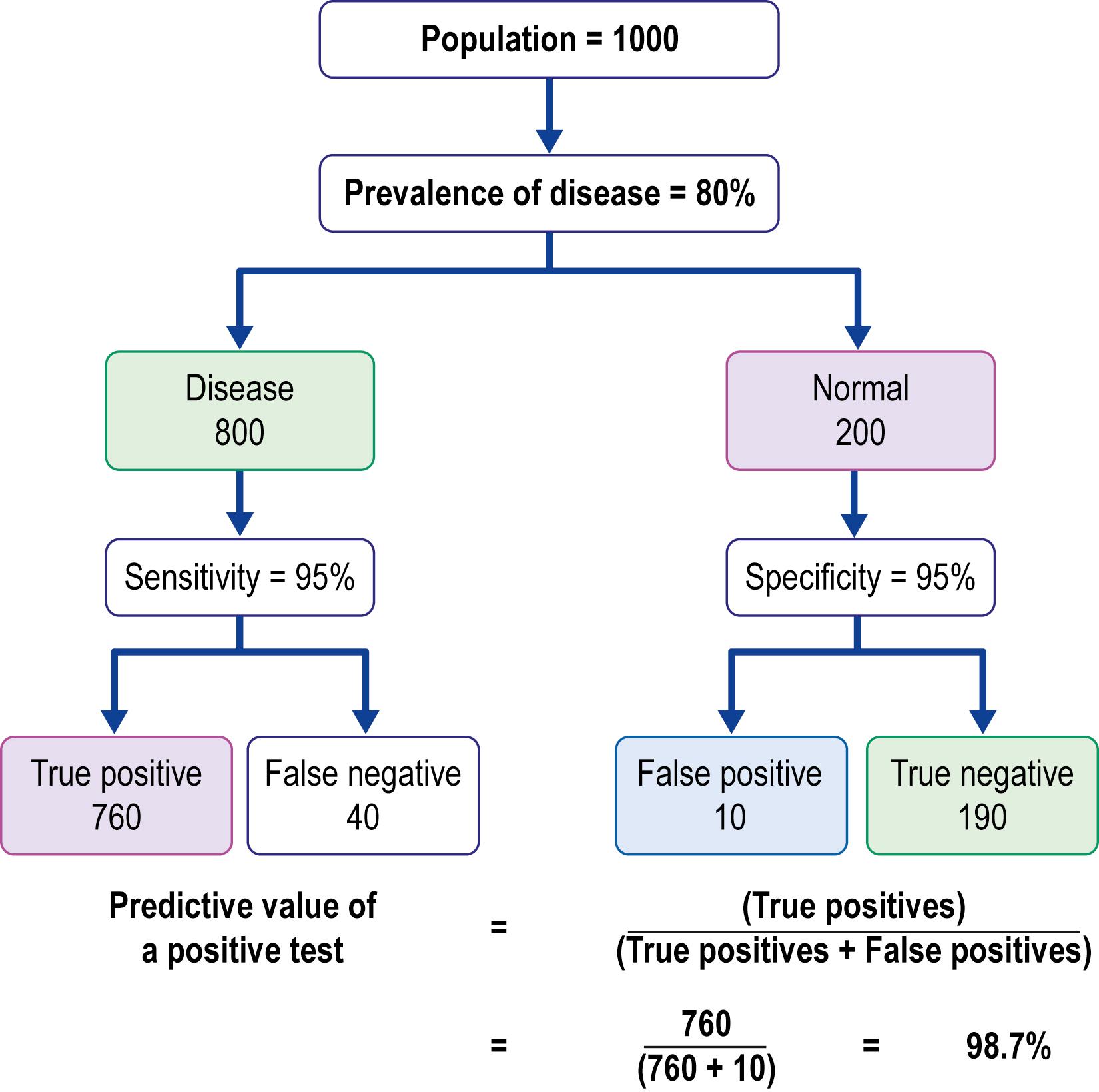
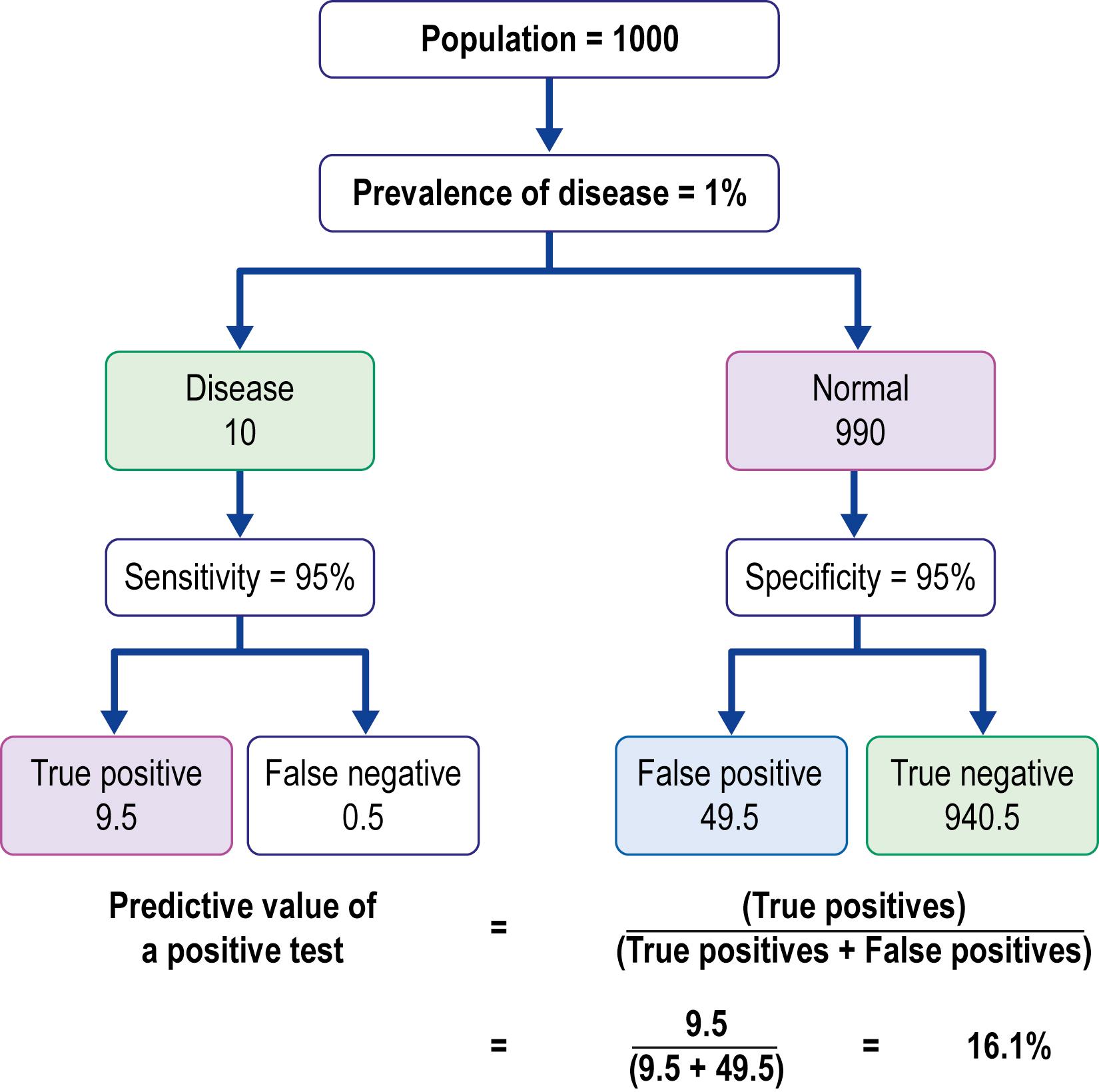
Bayes’ Theorem and the Predictive Value of A Positive Test

Bayes’ theorem states that the probability of a test demonstrating a true positive depends not only on the sensitivity and specificity of a test but also on the prevalence of the disease in the population being studied. The chance of a positive test being a true positive is markedly higher in a population with a high prevalence of the disease. In contrast, if a very sensitive and specific test is applied to a population with a very low prevalence of the disease, most positive tests will actually be false positives. The predictive value of a positive test is best explained by contrasting two examples ( Figs. 9.7 and 9.8 ). In both examples, the same test with a 95% sensitivity and a 95% specificity is applied to a population of 1000 patients. In Fig. 9.7 , the prevalence of the disease in the population is high (80%); in Fig. 9.8 , the prevalence is low (1%). In the population with a disease prevalence of 80%, 760 of the 800 patients with the disease will be correctly identified; of the 200 normals, 10 will be misidentified as abnormal (false positives). The predictive value of a positive test is defined as the number of true positives divided by the number of total positives. The total positives are the true positives added to the false positives. In Fig. 9.7 , the predictive value that a positive test is a true positive is 760/(760+10) =98.7%. Thus, in this example, in which the disease prevalence in the population is high, a positive test is extremely helpful in correctly identifying the patient as having the disease.

Fig. 9.7, Predictive value of a positive test: high prevalence of disease.

Fig. 9.8, Predictive value of a positive test: low prevalence of disease.

In the example in which the disease prevalence is 1% ( Fig. 9.8 ), of the 10 patients with the disease, 9.5 will be correctly identified. However, of the 990 normals, 49.5 will be misidentified as abnormal. Thus, the predictive value that a positive test is a true positive is 9.5/(9.5+49.5) =16.1%. This means that 83.9% of the positive results will actually be false! In this setting, in which the disease prevalence in the population is low, a highly sensitive and specific test is of absolutely no value.

Although this analysis may seem distressing, the good news is that EDX studies are generally performed on patients with a high index of suspicion for the disorder being questioned; hence, the prevalence of the disease is high. For instance, take the example of a patient referred to the EDX laboratory for possible carpal tunnel syndrome. If the patient has pain in the wrist and hand, paresthesias of the first four fingers, and symptoms provoked by sleep, driving, and holding a phone, the prevalence of carpal tunnel syndrome in patients with such symptoms would be extremely high. Thus, if EDX studies are performed and demonstrate delayed median nerve responses across the wrist, there is a very high likelihood that these positive tests are true positives. However, if the same tests are performed on a patient with back pain and no symptoms in the hands and fingers, the prevalence of carpal tunnel syndrome would be low in such a population. In this situation, any positive finding would have a high likelihood of being a false positive and would likely not be of any clinical significance.

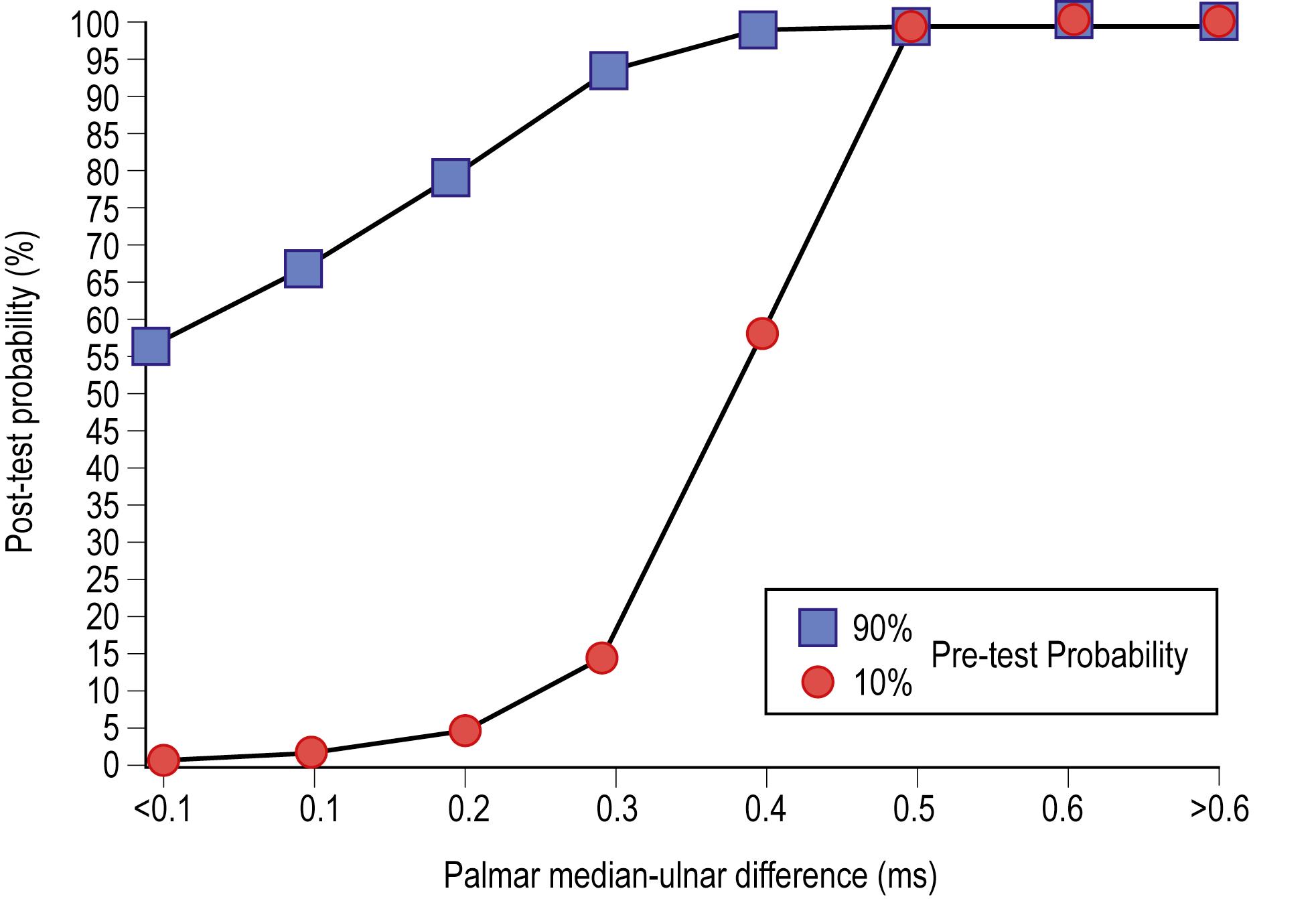
Less well appreciated is that the problem of a false positive in a population with a low prevalence of disease can be overcome by making the cutoff value more stringent (i.e., increasing the specificity). Take the example shown in Fig. 9.9 of the palmar mixed latency difference test in patients with suspected carpal tunnel syndrome. For this nerve conduction study, the latency for the ulnar palm-to-wrist segment is subtracted from the latency for the median palm-to-wrist segment, using identical distances. In normals, one expects there to be no significant difference. In patients with carpal tunnel syndrome, the median latency is expected to be longer than the ulnar latency. In this example, the post-test probability (i.e., the predictive value of a positive test) is plotted against different cutoff values for what is considered abnormal for patients in whom there is a high pre-test probability of disease and for those in whom there is a low pre-test probability. In the patients with a high pre-test probability of disease, a cutoff value of 0.3 ms (i.e., any value >0.3 ms is abnormal) achieves a 95% or greater chance that a positive test is a true positive. However, the same 0.3 ms cutoff in the low pre-test probability population results in only a 55% chance that a positive test is a true positive (and a corresponding 45% false-positive rate). These findings are in accordance with Bayes’ theorem wherein the chance of a positive test being a true positive depends not only on the sensitivity and specificity of the test but also on the prevalence of the disease in the population being sampled (i.e., the pre-test probability). However, if the cutoff value is increased to 0.5 ms, then the post-test probability that a positive test is a true positive jumps to greater than 95%, even in the population with a low probability of disease.

Fig. 9.9, Post-test probabilities (PostTPs) calculated with different pre-test probabilities (PreTPs).

Important clinical-electrophysiologic implications are as follows:

1.
Every EDX study must be individualized, based on the patient’s symptoms and signs and the corresponding differential diagnosis. When the appropriate tests are applied for the appropriate reason, any positive test is likely to be a true positive and of clinical significance.
2.
A test result that is minimally positive has significance only if there is a high likelihood of the disease being present, based on the presenting symptoms and differential diagnosis.
3.
A test that is markedly abnormal is likely a true positive, regardless of the clinical likelihood of the disease.
4.
An abnormal test, especially when borderline, is likely a false positive if the clinical symptoms and signs do not suggest the possible diagnosis.

You're Reading a Preview

Become a Clinical Tree membership for Full access and enjoy Unlimited articles

Become membership

If you are a member. Log in here

Bayes’ Theorem and the Predictive Value of A Positive Test

You're Reading a Preview

Related Posts

Appendix

Electrical Safety and Iatrogenic Complications of Electrodiagnostic Studies

Basics of Electricity and Electronics for Electrodiagnostic Studies

Approach to Pediatric Electromyography